Why Low Rank Adaptation Matters: A Closer Look at Its Impact on Machine Learning
Low Rank Adaptation (LoRA) is a fine-tuning technique designed to efficiently update and adapt large pre-trained models, such as language or diffusion models, without retraining them entirely. Low Rank Adaptation was proposed in 2021 by Edward Hu et al. They demonstrated that LoRA significantly reduces the number of trainable parameters and GPU memory requirements. But how is that possible? In this blog post, we will explore LoRA and understand the foundational principles underlying its concept.
1. Linear Algebra: Rank
Before we delve into Low Rank Adaptation, we first should be familar with rank of the matrix. The rank of a matrix is a fundamental concept in linear algebra that measures the dimensionality of the vector space spanned by its rows or columns. More intuitively, it represents the maximum number of linearly independent row vectors or column vectors in the matrix. Let’s see a few examples.
Matrix with Rank 1
- The second row \(A_2\) is equal to \(2A_1\)
- The third row \(A_3\) is equal to \(3A_1\)
- Each row is linearly dependent on the other rows \[ A = \begin{bmatrix} 1 & 2 & 3 \\ 2 & 4 & 6 \\ 3 & 6 & 9 \\ \end{bmatrix} \]
Matrix with Rank 2
- \(A_3 = A_1 + A_2\)
- The first two rows are linearly independent but the third row is the sum of the first two rows.
- Since the number of independent rows are two, \(rank(A)\) = 2 \[ A= \begin{bmatrix} 1 & 0 & 1 \\ 0 & 1 & 1 \\ 1 & 1 & 2 \\ \end{bmatrix} \]
Matrix with Full Rank
- Each row cannot be represented combination of other rows
- In other words, all rows are linearly independent to other rows
- \(rank(A)\) is full rank \[ \begin{bmatrix} 1 & 2 & 3 \\ 4 & 5 & 6 \\ 7 & 8 & 10 \\ \end{bmatrix} \]
Tip: You can use echelon forms to calculate the rank of the matrix.
2. Fine-tuning a Large Model
 Insights from Finetuning LLMs with Low-Rank Adaptation - Youtube
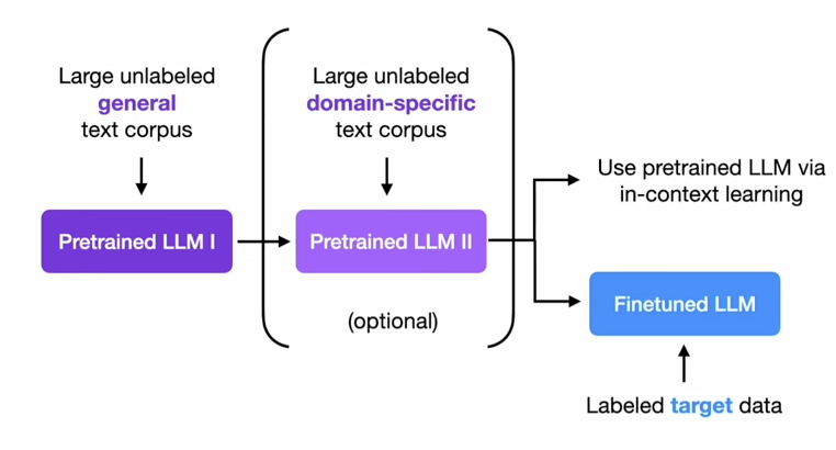
The GPT models follow a two-stage training approach that consists of pre-training on a large corpus of text in an unsupervised manner and fine-tuning on a specific task in a supervised manner. It’s obvious to think that pre-training is expensive and time-consuming. According to Nvidia documentation, training a GPT-2 model with 1.5 billion parameters takes roughly 100,000 GPU hours on 16 A100 GPUs. But what about fine-tuning?
Let’s first talk about full-fine tuning. Full-fine tuning is an approach to activate all the loaded parameters from pre-training. In other words, not freezing any layers of the model. The problem is the model is too large. Not only updating the parameters through epochs, but also loading the parameters into memory is expensive. For instance, GPT3 model has over 175 billion parameters and it requires 400GB of VRAM and takes minutes to load the model.
You may ask two questions reading above.
- Do we need to fine-tune all parameters?
- How expressive should the matrix updates be?
We will find out the answers to these questions in the next section.
3. Low Rank Adaptaion
Let’s answer the first question. Do we need to fine-tune all parameters? The answer is no. In the paper, the author said that LoRA freezes the pre-trained weights. Actually, it’s a common approach to freeze some of layers in fine-tuning. Traditionally, the lower layers are frozen and top layers or newly added layers (often called adapter) for specific task are unfrozen. This is because we assume that the model already learned the low level feature of the model in deeper layers. However, you shouldn’t confuse this approach with LoRA.
Restructuring the fine-tuning
First, let’s formulate fine-tuning process mathematically.
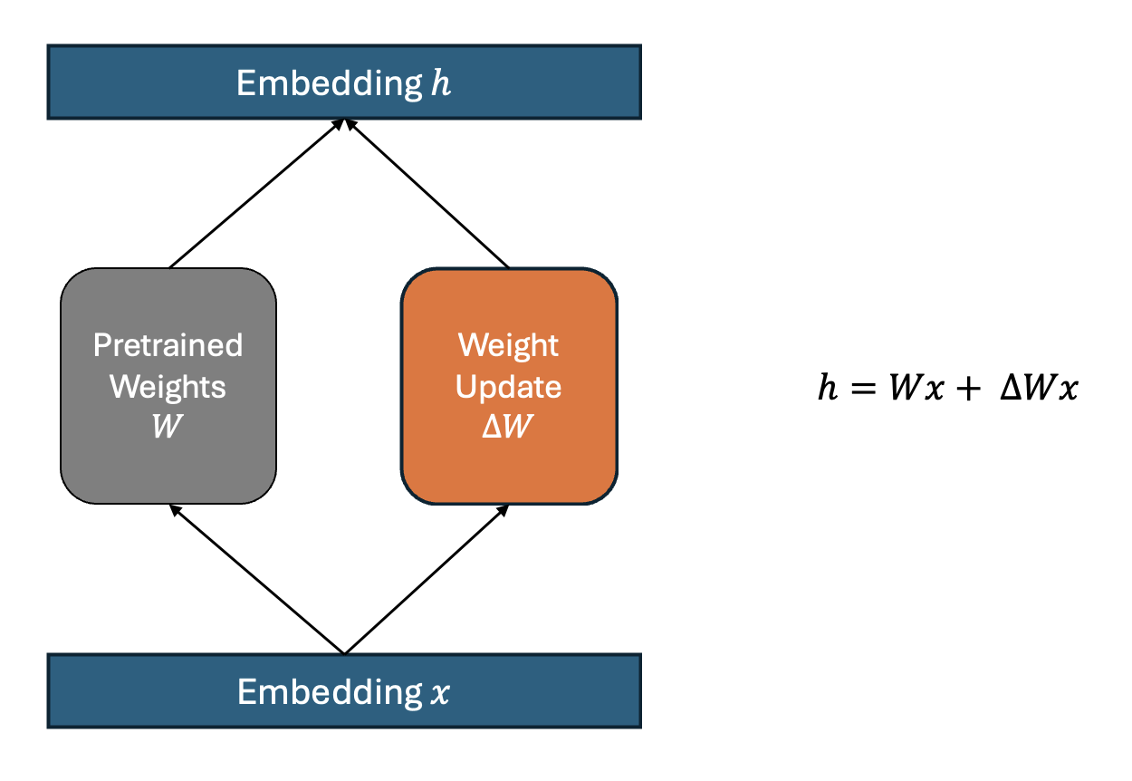
$$h = Wx + \Delta W$$Where:
- \(h\) is output embedding
- \(x\) is the input vector to the model
- \(W\) is original weight matrix from pre-trained model
- \(\Delta W\) represents the derivitive weight matrix from backpropagation
Instead of directly computing gradient descent of \(W\) to obtain \(\Delta W\), we can treat \(\Delta W\) as a independent set of weight. You can create the linear layer matrix that has the same dimension with \(W\).
It might come off not clear until you see the code.
class DeltaW(nn.Module):
    def __init__(self, in_dim, out_dim):
        super().__init__()
        self.weight = nn.Parameter(torch.randn(in_dim, out_dim)) #weight without bias

    def forward(self, x):
        x = x @ self.weight
        return x

# Model weight
class Model(nn.Module):
    def __init__(self):
        super().__init__()
        self.linear1 = nn.Linear(100, 1000) #let's say this layer is frozen and loaded
        self.delta_w1 = DeltaW(100, 1000)
        self.linear2 = nn.Linear(1000, 10) #frozen and loaded
        self.delta_w2 = DeltaW(1000, 10)

    def forward(self, x):
        x = self.relu(self.linear1(x) + self.delta_w1(x))
        x = self.linear2(x) + self.delta_w2(x)
        return x
In the above pseudo code, let’s say linear1 and linear2 layers are original pre-trained weights. We treat them as if these two layers are frozen. When you fine-tune this model, it will be identical to fine-tune the original model without delta_w1 and delta_w2.
Idea of LoRA
Again, fine-tuning \(\Delta W\) in the model is expensive. But what if the change in weights during model adaptation also has a low intrisic rank? This is the key hypothesis of LoRA. Instead of directly updating \(\Delta W\), we can decompose it into two smaller matrices, \(A\) and \(B\) such that:
$$\Delta W = A \times B$$Where \(A\) is a low-rank matrix and \(B\) projects it back to the original dimensions. The rank of these matrices is significantly lower than the original dimensions of \(\Delta W\), leading to a substantial reduction in the number of trainable parameters.
If you need wrap your head around, assume the weight matrix \(W\) of specific layer has dimensions of \(5000 \times 10000\), resulting in 50 million parameters in total. If you decompose \(W\) into \(A\) and \(B\) where \(A\) has dimensions of \(5000 \times 8\) and \(B\) has dimensions of \(8 \times 10000\), then the rank of \(W\) is 5000. Combined, these matrices account for only \(80,000 + 40,000 = 120,000\) parameters, which is 400 times fewer than the 50 million parameters involved in standard fine-tuning.
How to determine rank \(r\)
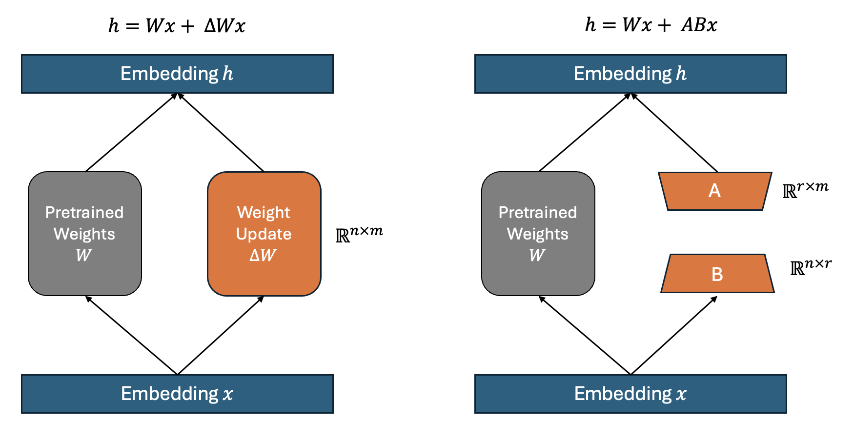 The right figure in the above image shows LoRA approach. Here, \(r\) denotes the rank of \(\Delta W\) and is a hyperparameter that determines the rank of \(A\) and \(B\). While I was reading the paper, I was confused because \(r\) represents the smaller dimension of \(A\) and \(B\), and also represents the rank of \(\Delta W\). You need to understand the principle of low-rank factorization. The goal of Low-Rank Matrix Factorization is to approximate a high-dimensional matrix as a product of two smaller matrices \(A\) and \(B\) by constraining the dimension of \(A\) and \(B\) to \(\mathbb R^{n \times r}\) and \(\mathbb R^{r \times m}\) respectively. \(r\) is determined the rank of \(\Delta W\). The motivation of low-rank approximation is that we keep the information of the original matrix by keeping rank.
Think about this. The best way to reduce the number of parameters is just setting \(r\) as low as possible. The number of parameters would be as follows when \(\Delta W\) has dimension of \(5000 \times 10000\),
- \(r\) = 1, then num_param = 15000
- \(r\) = 2, then num_param = 30000
- \(r\) = 3, then num_param = 45000
Let me ask again: why can just set \(r\) to 1? This would result in a model with only 15,000 parameters. The reason is that setting \(r\) below the rank of \(\Delta W\) can lead to the loss of significant information. Here, the critical factor is the rank of the matrix \(\Delta W\). So, can we determine the rank of \(\Delta W\) and shape \(A\) and \(B\) accordingly? We can but computing the rank of \(\Delta W\) for all layers is intractable. In the paper the value of \(r\) is fixed at several predetermined levels: 1, 2, 8, 64, … , up to 1024. So basically, the paper shows the investigation of the value of \(r\) to find what the rank of \(\Delta W\) so we can decompose \(\Delta W\) into \(A\) and \(B\).
LoRA Implementation
Let’s write the implementation of LoRA based on what we learned so far. There are a few things to note for implementation.
- \(A\) is initialized with a Gaussian distribution
- \(B\) is initialized with zero
- \(\alpha\) is used for scaling the \(\Delta W\)
import torch.nn as nn

class LoRALayer(nn.Module):
    def __init__(self, in_dim, out_dim, rank, alpha):
        super().__init__()
        std_dev = 1 / torch.sqrt(torch.tensor(rank).float())
        self.A = nn.Parameter(torch.randn(in_dim, rank) * std_dev)
        self.B = nn.Parameter(torch.zeros(rank, out_dim))
        self.alpha = alpha

    def forward(self, x):
        x = self.alpha * (x @ self.A @ self.B)
        return x
With this implementation, we can replace pretrained linear layers with LoRA layers.
Conclusion
Low Rank Adaptation (LoRA) offers an efficient way to fine-tune large pre-trained models by reducing the number of trainable parameters and memory requirements. It utilizes concepts from linear algebra to maintain model effectiveness while lowering computational demands. This method allows for deeper models to be fine-tuned more easily and with fewer resources. Overall, LoRA is a crucial advancement that enhances the usability and efficiency of machine learning models.