 Graph structures have been applied in many scientific fields, such as biology, computer science, and social network analysis. With the increasing popularity of machine learning, the graph representation learning (GRL) paradigm has emerged as effective methods. One example is the Graph Convolutional Network (GCN), which has shown remarkable success in tasks like node classification, graph generation and clustering by effectively capturing the complex relationships in graph data. GRL is also making big waves in modern computer vision.
You might wonder how GRL can be used in modern computer vision. The potential of graphs isn’t just about finding paths from point A to point B. For instance, you can restructure an image into a graph, transforming pixels into nodes and their relationships into edges. That’s not it. You can even restructure a complex label for an image into a graph and use it for graph learning. In this article, we will talk about how graph representation learning can be used in modern computer vision. We will also cover a pratice of graph representation learning using Pytorch.
Graph Theory and Terminology
Mathematically, a graph is a pair \(G = (V ,E)\) where \(V\) is a set of vertices and \(E\) is a set of ordered pairs of vertices called edges. In a weighted graph, graph can be represented \(G = (V ,E, W)\) where \(W\) is a adjecency matrix, \(W \in \mathbb{R}^{n \times n}\). \(W_{ij}=0\), if there is no edge between vertices \(i\) and \(j\). In some graph theory books, \(W_{ij} = \infty \) when there is no edge between vertices \(i\) and \(j\). However, in this article, we will stick to the former definition.
Adjacency Matrix
There are many representations for graph strucuters such as Adjacency Matrix, Adjacency Matrix, and Edge List, and Compressed Sparse Row. In this article, we only cover Adjacency Matrix. See an example in the below image to understand how weighted directed graph can be represented in Adjacency Matrix.
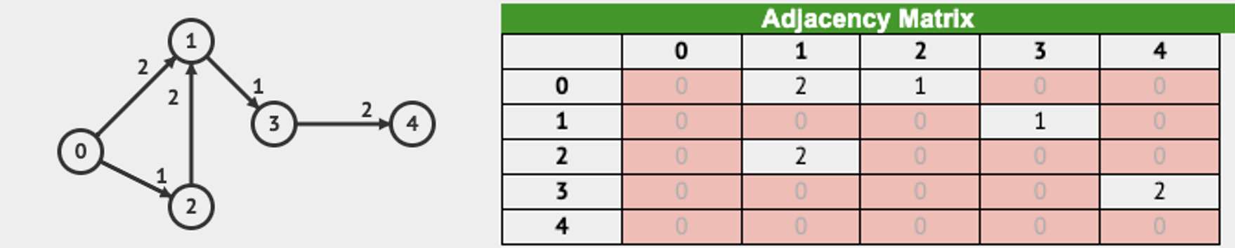
Image to Graph
We learned mathemtical background of graph theory. But still you might not clear how graph can be applied to computer vision i.e., image to graph. Let’s recall what a neural network does. Simply put, a neural network can be viewed as an encoder that maps data to low dimensional representation for further tasks. So the encoder will function if the data is represented in a vector space. The question is how we represent image to graph? Commonly, there are two types of graph representation.
- Pixel graph representation
- Semantic graph representation
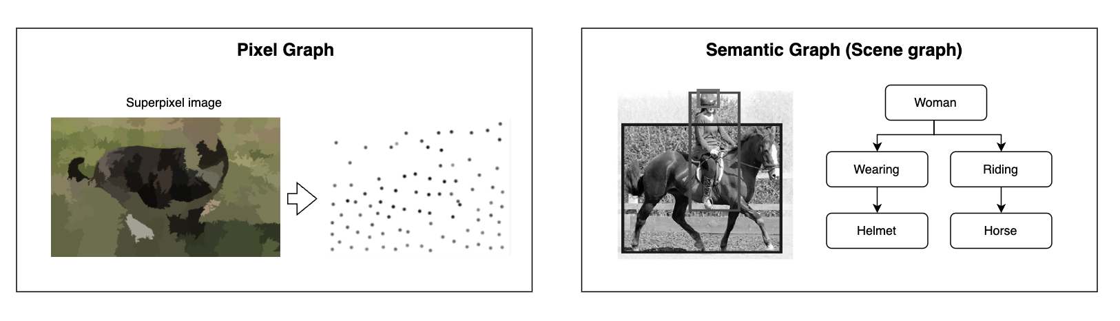
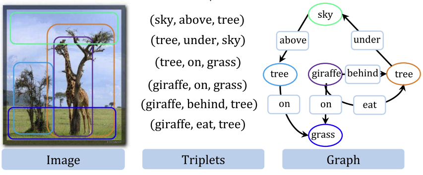
Pixel graph representation is very intuitive. Pixel graph representation converts an image into a graph structure, where pixels or groups of pixels are treated as nodes, and edges represent relationships between them. Superpixeling is often used to reduce the redundant pixel-level data (node) as an image compression. Semantic graph representation can be referred to as an object-based graph or label graph. The objects in an image generally have some semantic relationships between them (unless it’s a random white noise image). The goal of semantic graph representation is to structure and model the semantic relationships between objects, capturing contextual and relational information in a structured manner.
Graph Convolutional Network
 Graph convolutional neural networks https://mbernste.github.io/posts/gcn/
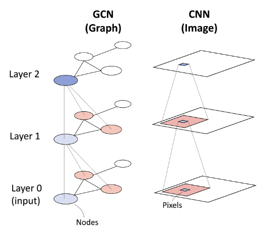
Convolution works well on images as it aggregate neighboring features. In the same way, the graph convolution aggregate information from a node’s neighbors. The difference is that standard convolutions operate on local Euclidean in an image, graph convolution extend this concept to non-Euclidean data, where nodes are connected by an adjacency matrix. Let’s take a look at mathmatical definition of graph convolution.
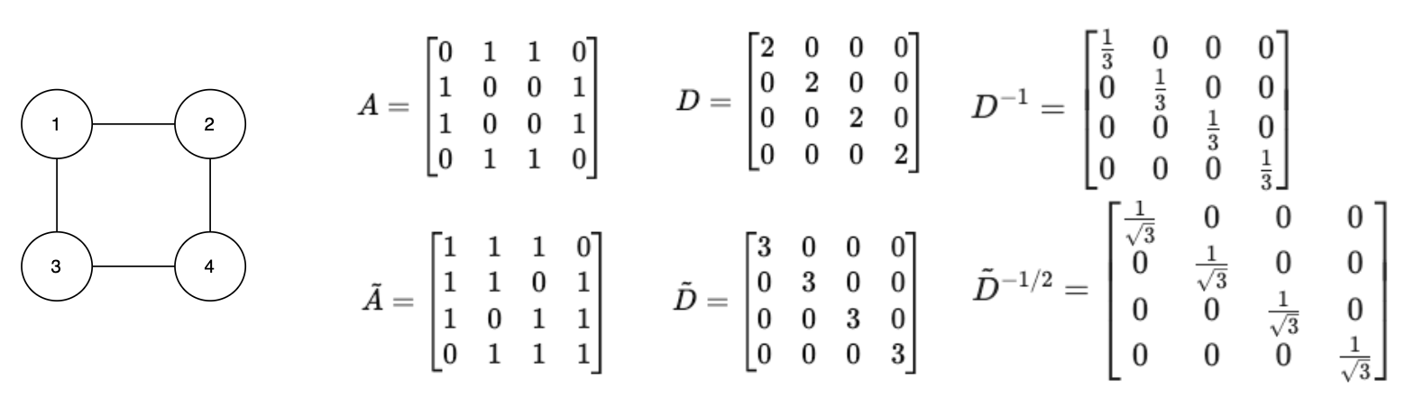
\[ H^{(l+1)} = \sigma \left( \tilde{D}^{-1/2} \tilde{A} \tilde{D}^{-1/2} H^{(l)} W^{(l)} \right) \]- \(H^{(l)} \in \mathbb{R}^{n \times d}\) is the feature matrix at layer \(l\), where each row is a node’s feature vector
- \(\tilde{A} = A + I\) is the adjacency matrix with identity matrix (self-loops)
- \(\tilde{D}\) is the degree matrix of \(A + I\)
- \(W^{(l)} \in \mathbb{R}^{d \times d}\) is the weight matrix at layer \(l\)
- \(\sigma\) is the non-linear function (e.g., ReLU)
The key concept of convolution is to aggregate information from neighbors. Let’s see how the equation is derived. It starts from \(H' = AH\), which means that each node’s new feature representation is obtained by summing the feature vectors of its direct neighbors. However, there are two major issues:
- It doesn’t include the node’s own features
- It doesn’t normalize the contribution of neightbors, which can lead to exploding gradient or vanishing gradient
To include the noide’s own features, we can add self-loops to the adjacency matrix \(\tilde{A} = A + I\) such that \(H' = \tilde{A}H\). To normalize the contribution of neighbors, we can use the degree matrix \(\tilde{D} = D\). To normalize the feature aggregation, we introduce degree matrix \(\tilde{D} = \sum_j\tilde{A}_{ij}\). The natual normalization approach is \(H' = \tilde{D}^{-1}\tilde{A}H\) because each node averages its neighbors’ contributions. However, when normalizing adjacency matrix, the symmetric normalization approach is used such that \(H' = \tilde{D}^{-1/2}\tilde{A}\tilde{D}^{-1/2}H\). The reason is \(\tilde{D}^{-1}\tilde{A}\) only ensures row noalization and \(\tilde{A}\tilde{D}^{-1}\) only ensures column normalization. The symmetric normalization approach is more stable.
Multi-label Classification with GCN
Now that we understand the definition of the graph convolution operation, let’s explore one of its most popular use cases. Imagine a random image of a tennis game. In this image, you’d likely see a person holding a racket and attempting to hit a tennis ball. These objects are not just randomly placed in the scene—they are inherently connected. If there’s a tennis ball, it’s highly likely that a racket is nearby, and if there’s a racket, it’s probably being held by a person.
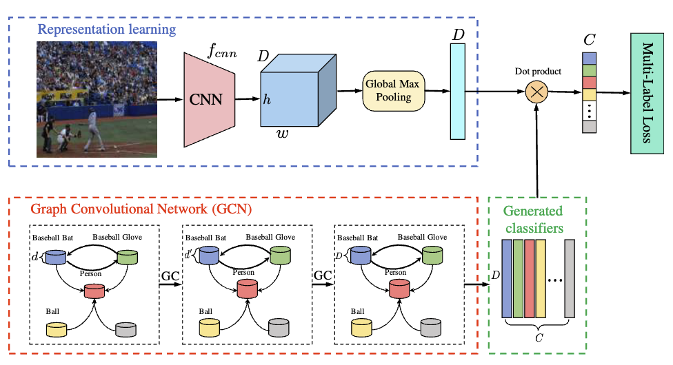
Multi-Label Image Recognition With Graph Convolutional Networks was published in 2019 and cited more than 1k. The authors use GCN to capture semantic dependencies between object labels in multi-label image recognition. Yes, this approach uses semantic graph representation. Instead of treating labels as independent categories, their approach models them as nodes in a directed graph, where edges represent co-occurrence relationships learned from data. Then, are they ignoring images? Of course not, they use CNN to encode the image features.
Code Review
The below code is the source code of the ML-GCN proposed by the authors.
import torchvision.models as models
from torch.nn import Parameter
from util import *
import torch
import torch.nn as nn

class GraphConvolution(nn.Module):
    def __init__(self, in_features, out_features, bias=False):
        super(GraphConvolution, self).__init__()
        self.in_features = in_features
        self.out_features = out_features
        self.weight = Parameter(torch.Tensor(in_features, out_features))
        if bias:
            self.bias = Parameter(torch.Tensor(1, 1, out_features))
        else:
            self.register_parameter('bias', None)
        self.reset_parameters()

    def reset_parameters(self):
        stdv = 1. / math.sqrt(self.weight.size(1))
        self.weight.data.uniform_(-stdv, stdv)
        if self.bias is not None:
            self.bias.data.uniform_(-stdv, stdv)

    def forward(self, input, adj):
        support = torch.matmul(input, self.weight)
        output = torch.matmul(adj, support)
        if self.bias is not None:
            return output + self.bias
        else:
            return output

    def __repr__(self):
        return self.__class__.__name__ + ' (' \
               + str(self.in_features) + ' -> ' \
               + str(self.out_features) + ')'


class GCNResnet(nn.Module):
    def __init__(self, model, num_classes, in_channel=300, t=0, adj_file=None):
        super(GCNResnet, self).__init__()
        self.features = nn.Sequential(
            model.conv1,
            model.bn1,
            model.relu,
            model.maxpool,
            model.layer1,
            model.layer2,
            model.layer3,
            model.layer4,
        )
        self.num_classes = num_classes
        self.pooling = nn.MaxPool2d(14, 14)

        self.gc1 = GraphConvolution(in_channel, 1024)
        self.gc2 = GraphConvolution(1024, 2048)
        self.relu = nn.LeakyReLU(0.2)

        _adj = gen_A(num_classes, t, adj_file)
        self.A = Parameter(torch.from_numpy(_adj).float())
        # image normalization
        self.image_normalization_mean = [0.485, 0.456, 0.406]
        self.image_normalization_std = [0.229, 0.224, 0.225]

    def forward(self, feature, inp):
        feature = self.features(feature)
        feature = self.pooling(feature)
        feature = feature.view(feature.size(0), -1)

        inp = inp[0]
        adj = gen_adj(self.A).detach()
        x = self.gc1(inp, adj)
        x = self.relu(x)
        x = self.gc2(x, adj)

        x = x.transpose(0, 1)
        x = torch.matmul(feature, x)
        return x

    def get_config_optim(self, lr, lrp):
        return [
                {'params': self.features.parameters(), 'lr': lr * lrp},
                {'params': self.gc1.parameters(), 'lr': lr},
                {'params': self.gc2.parameters(), 'lr': lr},
                ]

def gen_adj(A):
    D = torch.pow(A.sum(1).float(), -0.5)
    D = torch.diag(D)
    adj = torch.matmul(torch.matmul(A, D).t(), D)
    return adj

def gcn_resnet101(num_classes, t, pretrained=False, adj_file=None, in_channel=300):
    model = models.resnet101(pretrained=pretrained)
    return GCNResnet(model, num_classes, t=t, adj_file=adj_file, in_channel=in_channel)
The first thing we should look at is that the forward function of GCNResnet. It takes feature and inp, which is word embedding. The authors stated that they adopted 300-dim GloVe for label representation. But why didn’t they just uses one hot encoding for the labels? One-hot encoding represents labels as discrete, independent categories, meaning it does not capture any semantic relationships between them. In contrast, GloVe embeddings encode words in a continuous space where semantically similar words have closer representations.
The next thing we look is adj = gen_adj(self.A).detach() in the forward function. Here, self.A is the adjacency matrix. The adjacency matrix is processed using gen_adj() function to generate the normalized adjacency matrix, \( \hat A = \tilde{D}^{-1/2} \tilde{A} \tilde{D}^{-1/2}\). The ML-GCN uses two graph convolutional layers. self.gc1(inp, adj) and self.gc2(x, adj). The inp represents the word embedding \(H^{l}\). The forward function of GraphConvolution performs \(H^{l+1} = \hat AH^{l}W^{l}\)
Lastly, the graph embedding and image embedding are multiplied to generate the final multi-label predictions by torch.matmul(feature, x). The output of the GCNResnet has a dimension of \((\text{batch}, \text{number of classes})\), where each entry represents the probability score for each class in the image. The network is trained using multilabel classification loss (BCE) funciton.
Conclusion
We dipped our toes into key concepts of graph theory and how graph representation learning finds its way into the field of computer vision. We explored Graph Convolutional Networks (GCNs) and their application to multi-label image classification. Graph learning continues to gain momentum in academic research. What we learned is just the tip of the adjacency matrix, but graph learning extends far beyond classification. Researchers have been unlocking breakthroughs in semantic segmentation, action recognition, person re-identification, object tracking, and visual question answering. Plus, with graph transformers making waves in both NLP and computer vision, graph representation learning is gearing up for even bigger roles. Thanks for reading!
Reference
- Graph Representation Learning Meets Computer Vision: A Survey
- Multi-Label Image Recognition with Graph Convolutional Networks, CVPR 2019
- https://mbernste.github.io/posts/gcn/
- https://www.youtube.com/watch?v=CwHNUX2GWvE
- https://math.stackexchange.com/questions/3035968/interpretation-of-symmetric-normalised-graph-adjacency-matrix