 When I first started studying reinforcement learning, I was intimidated by the amount of mathematical background required to understand even the basic concepts. Terms like “Markov property,” “Bellman equation,” and “Q-learning” felt abstract and overwhelming. In this blog post, we will walk through these foundations step by step, starting from probability basics and building up toward deep reinforcement learning. Specifically, we will cover: 1) Markov decision process (MDP) 2) Value function, 3) Q-learning, and 4) Deep Q-learning (DQN). After reading this post, you will understand how reinforcement learning builds from the Markov property to value-based methods, and finally to Deep Q-Learning.
1. Markov Property
The Markov Property is a fundamental concept in probability theory that states that the future state of a process depends only on its current state and not on the sequence of events that preceded it.
1.1. Markov Process
A Markov process (markov chain) is a special type of random process that satisfies the Markov property. The Markov property states that the future state of the process depends only on the current state and not on any previous states. Formally:
\[ P(S_{t+1} = s' \mid S_t = s, S_{t-1} = s_{t-1}, \ldots, S_0 = s_0) = P(S_{t+1} = s' \mid S_t = s) \]Where
- \( S_t \) represents the state of at time \( t \).
- \(P(S_{t+1} = s' \mid S_t = s)\) denotes state probability.
Let’s think how Markov came up with this modeling. We can assume that the stock price \(S_t+1\) might depend on previous stock price \(S_{t}, S_{t-1}, \cdots, S_{0}\). But Markov said no! The stock price at the next time step \(X_{t+1}\)only depends on the current price \(S_t\) and not on the entire history of previous prices. Markov believed that in many real-world processes, including finance, weather prediction, and other systems, the most recent information captures all the relevant data needed to predict future behavior. This assumption simplifies modeling because we don’t need to consider complex historical dependencies.
1.2. State Transition Matrix
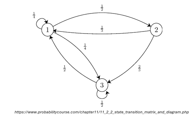
The above figure is an example of state transition diagram used to visualize markov chain problem. The number between states is a transition probability \(P(S_{t+1} = s' \mid S_t = s)\). Let’s say we start from state 1 (i.e. \(t=0\) and \(s=1\)). The transition probability \(P(S_{1} = 2 \mid S_{0} = 1)\) is 1/3. The example diagram can be represented as a state transition matrix:
\[ P = \begin{bmatrix} \frac{1}{4} & \frac{1}{2} & \frac{1}{4} \\ \frac{1}{3} & 0 & \frac{2}{3} \\ \frac{1}{4} & 0 & \frac{1}{2} \end{bmatrix} \]State transition matrix follows a property as follows:
\[\sum_{k=1}^{r} p_{ik} = \sum_{k=1}^{r} P(S_{t+1} = k \mid S_t = i) = 1\]This means the sum of probabilities of transitioning to next state is equal to 1.
Using the transition matrix, we can sample a sequence of states based on the transition probabilities:
- Example Sequence 1: \( 1 \rightarrow 2 \rightarrow 3 \rightarrow 3 \rightarrow 1 \)
- Example Sequence 2: \( 1 \rightarrow 1 \rightarrow 3 \rightarrow 1 \)
This type of sampling process is known as a random walk. In a random walk, the next state is chosen based on the current state and its associated transition probabilities.
1.3. Markov Decision Process
A Markov Decision Process (MDP) forms the foundation of reinforcement learning. It is an extension of a Markov process that introduces actions and rewards, enabling decision-making in stochastic environments.Reinforcement learning is based on MDP. An MDP provides a mathematical framework for modeling decision-making problems where an agent interacts with an environment to maximize a cumulative reward over time.
An MDP consists of parameters \( (S, A, P, R, \gamma) \), where:
- \( S \): The set of possible states in the environment.
- \( A \): The set of possible actions that the agent can take.
- \( P(s' \mid s, a) \): The transition probability function, which defines the probability of moving to state \( s' \) given that the agent takes action \( a \) in state \( s \).
- \( R(s, a) \): The reward function, which defines the immediate reward received after taking action \( a \) in state \( s \).
- \( \gamma \): The discount factor, a value between 0 and 1 that represents the importance of future rewards.
The action at each time stamp \(a_t \in A\) will be determined by a policy \(\pi (a|s)\).
Based on a policy, an agent generates a sequence of states and actions \(\tau\), called “state and action trajectory”. The trajectory is expressed as \(\tau : (s_0, a_0, s_1, a_1, \ldots, s_t, a_t)\).
The goal of MDP is to maximize a cumulative reward, called “expected return”. Technically, the expected return \( G_t \) represents the cumulative discounted reward starting from time step \( t \):
\[ G_t = R_{t+1} + \gamma R_{t+2} + \gamma^2 R_{t+3} + \ldots = \sum_{k=0}^{\infty} \gamma^k R_{t+k+1} \]Here, \(R_{t+1}\) is the reward received after the transition from state \(S_t\) to state \(S_{t+1}\). \(t\) is time stamp, don’t be confused with state.
2. Background for Reinforcement Learning (RL)
2.1. Value Function
The value function measures how good it is to be in a state, under a specific policy \(\pi\). Again, the goal is to maximize the expected return \( G_t \). To maximize the return, we aim to find an optimal stochastic policy \(\pi(a|s)\). The value function \(V^{\pi}\) represents the expected return when starting from state \(s\) and following policy \(\pi\):
\[ V^\pi(s) \triangleq \mathbb{E}_\pi \left[ G_t \mid S_t = s \right] = \mathbb{E}_\pi \left[ \sum_{k=0}^\infty \gamma^k R_{t+k+1} \mid S_t = s \right] \]This value function has recursive relationship because of the nature of the return \(G_t\).
\[G_t = R_{t+1} + \gamma G_{t+1}\]Then, we can rewrite the value function using this recursive chracteristic of the return. This recursive relationship is known as the Bellman equation.
\[ V^\pi(s) = \mathbb{E}_\pi \left[ R_{t+1} + \gamma G_{t+1} \mid S_t \right] \]We are not done yet. I want \(V^{\pi}\) to be both right and left sides of equation. We use law of iterated expectations:
\[ \mathbb{E}_\pi \left[ G_{t+1} | S_t = s \right] = \mathbb{E}_\pi [\mathbb{E}_\pi [G_{t+1} | S_{t+1}] | S_t = s ] \]But by the definition of the value function, we know:
\[ V^{\pi}(s_{t+1}) = \mathbb{E}_{\pi} [G_{t+1} | S_{t+1}] \]Now, replacing this in the earlier equation:
\[ V^\pi(s) = \mathbb{E}_\pi \left[ R_{t+1} + \gamma V^\pi(S_{t+1}) \mid S_t = s \right]. \]2.2. State-Action value function (Q function)
The value function \(V^{\pi}(s)\) is missing something. It doesn’t tell us which action \(a\) is best to take in that state. Therefore, we need to define a new function called “state-action value function or Q function.
\[ Q^\pi(s, a) \triangleq \mathbb{E}_\pi \left[ \sum_{k \geq 0} \gamma^k R_{t+k} \mid S_t = s, A_t = a \right] \\ = \mathbb{E}_\pi \left[ R_{t+1} + \gamma V^\pi(S_{t+1}) \mid S_t = s, A_t = a \right] \]The Q function \(Q^{\pi}(s,a)\) explicitly conditions on both state and action, which provides a more granular view of the agent’s behavior and allows for better decision-making. Let’s break the equation into two terms.
We denote the immediate reward expectation as \(r(s,a)\):
\[ \mathbb{E}_\pi[R_{t+1} | S_t = s, A_t = a] = r(s,a). \]The expected discounted value function of the next state \(S_{t+1}\) can be rewritten with the transition probability \(P(s'|s,a)\) where \(s'\) is next state of \(s\) (for simplicity \(s'\) will be used instead of \(S_{t+1}\)):
\[ \mathbb{E}_\pi \left[ \gamma V^\pi(S_{.t+1}) \mid S_t = s, A_t = a \right] = \gamma \sum_{s'}P(s'|a,s)V^{\pi}(s') \]By combining these two terms:
\[ Q^{\pi}(s,a) = \mathbb{E}_\pi \left[ R_{t+1} + \gamma V^\pi(S_{t+1}) \mid S_t = s, A_t = a \right] = r(s,a) + \gamma \sum_{s'}P(s'|a,s)V^{\pi}(s'). \]However, the euqation is not respect to the policy \(\pi(a|s)\) yet. Therefore, we substitute \(V^{\pi}(s')\) by writing relationship between value function \(V^{\pi}\) and Q function \(Q^\pi\).
\[V^\pi (s) = \mathbb{E}_\pi \left[ Q^\pi (s,a) \mid S_{t} = s \right]\]We can rewrite the expected Q-value over all possible action \(A_t\).
\[V^\pi(s) = \sum_a \pi (a|s)Q^\pi (s,a)\]Thus, we can replace \(V^{\pi}(s')\) in equation of \( Q^\pi(s, a) \) as:
\[ Q^\pi(s, a) = r(s, a) + \gamma \sum_{s'} P(s' \mid a, s) \sum_{a'} \pi(a' \mid s') Q^\pi(s', a') \]2.3. Bellman Optimality Equation for \( Q^*(s, a) \)
The optimal Q-function, denoted as \( Q^*(s, a) \), follows a recursive relationship similar to the Bellman equation for \( V^*(s) \). The optimal Q-function satisfies:
\[ Q^*(s, a) = r(s, a) + \gamma \sum_{s'} P(s' \mid s, a) \max_{a'} Q^*(s', a') \]This equation states that the optimal Q-value for state-action pair \( (s, a) \) is the immediate reward plus the discounted expected future rewards assuming that the agent always follows the best possible action thereafter.
- Instead of averaging over actions as in the policy evaluation step, we now maximize over the next possible actions.
- This is a key component in value iteration, where the agent repeatedly updates \( Q^*(s, a) \) until convergence.
3. How We Classify RL Methods
Before we jump into specific RL algorithms, we better know that there are a few categories we can label those algorithms.
3.1. Model-based vs. Model-free methods
Here the model does not mean a statistical or machine learning model. It means a representation of the environment’s dynamics. Technically, a model refers two parts: transition function \(P(s'|s,a)\) and reward function \(R(s,a)\).
- Model-Based methods assume the agent can learn the environment’s dynamics
- i.e., estimate value \(V(s)\) or \(Q(s,a)\) based on envrionment \(P(s'|s,a)\) and \(R(s,a)\).
- In autonomous driving, the car is equipped with a high-definition 3D map, traffic rules, and a physics simulator. The system can plan an entire route in advance without physically driving it first.
- Model-Free methods skip building the environment model and learn directly from experience
- i.e., estimate \(V(s)\) or \(Q(s,a)\) directly from samples without knowing \(P(s'|s,a)\) and \(R(s,a)\).
- In autonomous driving, They don’t have a map, no traffic rules book, no physics simulator. Just the ability to try actions (steering, braking, accelerating) and see what happens.
3.2. Value-based vs. Policy-based methods vs. Actor-critic
- Value-Based methods focus on learning a value function (\(V(s)\) or \(Q(s,a)\)).and derive a policy from it
- Policy-based method skip value functions and directly learn the policy \(\pi (a|s)\).
- Actor–Critic methods are hybrids where the agent learn both a policy (actor) and a value function (critic).
3.3. On-Policy vs. Off-Policy
- On-Policy methods learn from the actions actually taken by the current policy.
- Off-Policy methods learn the value of a different policy than the one used to collect data.
3.4. Existing RL algorithms categorization
| Algorithm | Model-Based / Model-Free | Value-Based / Policy-Based / Actor–Critic | On-Policy / Off-Policy |
|---|---|---|---|
| Dynamic Programming method | Model-Based | Value-Based | On-Policy |
| Monte Carlo method | Model-Free | Value-Based | On-Policy |
| SARSA | Model-Free | Value-Based | On-Policy |
| Q-Learning | Model-Free | Value-Based | Off-Policy |
| A2C (Advantage Actor–Critic) | Model-Free | Actor–Critic | On-Policy |
| PPO (Proximal Policy Optimization) | Model-Free | Actor–Critic | On-Policy |
4. Q-learning
The goal of Q-learning is to learn the optimal action-value function \(Q^*(s,a)\) that maximizes the agent’s expected cumulative discounted reward:
\[ \max_{\pi} \mathbb{E}_{\pi} \left[ \sum_{t=0}^{\infty} \gamma^{t} R_{t+1} \right] = \max_{\pi}Q^\pi(s,a) = Q^*(s,a). \]If we know \(Q^* (s,a)\) from learning process, the optimal value for each state-action pair, we can derive the optimal policy \(\pi\):
\[ \pi^*(s) = \arg\max_{a} Q^*(s, a). \]This is known as the greedy policy with respect to \( Q^*(s, a) \). This is why Q-learning is called value-based method. Value-based methods learn a value function \(Q(s,q)\) and derive a policy \(\pi^*(s)\).
Now, let’s get back to the Bellman Optimality Equation.
\[ Q^*(s, a) = r(s, a) + \gamma \sum_{s'} P(s' \mid s, a) \max_{a'} Q^*(s', a') \]Q-learning is a model-free method so we don’t know \(P\). We can replace the expectation with a sample. If at time \(t\) we take action \(a_t\) in state \(s_t\), observe reward \(r_{t+1}\), and next state \(s_{t+1}\), then:
\[ y_t = r_{t+1} + \gamma \max_{a'} Q(s_{t+1}, a') \]\(y\) is called the TD (temporal difference) target — it’s a single Monte Carlo sample of the expectation in the Bellman equation.
We want \(Q(s_t, a_t)\) to move toward the target \(y_t\). The general incremental update form is:
\[ Q(s_t, a_t) \leftarrow Q(s_t, a_t) + \alpha [y_t - Q(s_t, a_t)] \]where \([\text{y} - Q(s_t, a_t)]\) is called Bellman error. By substituting the TD target:
\[ Q(s_t, a_t) \leftarrow Q(s_t, a_t) + \alpha \left[ r_{t+1} + \gamma \max_{a'} Q(s_{t+1}, a') - Q(s_t, a_t) \right] \]4.1.Epsilon Greedy Strategy
The problem of the policy \(\pi^*(s)\) derived from the \(Q\) is that it’s determinititic, which means the agent repeatedly chooses the same action and may get stuck in a local optimum, never discovering better alternatives. To mitigate this, we introduce randomness in action selection through the ε-greedy strategy. The ε-greedy policy selects actions according to:
\[ a = \begin{cases} \text{random action}, & \text{with prob. } \varepsilon \\ \arg\max_{a} Q(s, a), & \text{with prob. } 1 - \varepsilon \end{cases} \]Here, the parameter \(\epsilon \in [0,1]\) controls the balance between exploration (trying random actions to gather more information) and exploitation (choosing the current best-known action).
4.2. Q-learning algorithm flow
Initialize
- For all states \(s\) and actions \(a\), set \(Q(s,a)\) (e.g., to 0).
- Choose:
- Learning rate \(\alpha \in (0,1]\)
- Discount factor \(\gamma \in [0,1)\)
- Exploration rate \(\varepsilon \in [0,1]\)
For each episode (repeat until convergence or max episodes):
- Reset environment; get initial state \(s\).
- Loop (until \(s\) is terminal):
- Action selection (behavior policy):
- With probability \(\varepsilon\), choose a random action.
- Otherwise, choose \(a = \arg\max_{a'} Q(s,a')\). (ε-greedy)
- Act & observe: execute \(a\); observe reward \(r\) and next state \(s'\).
- Target (off-policy, greedy): \[ y_t = r + \gamma \max_{a'} Q(s', a') \]
- Update (TD step): \[ Q(s,a) \leftarrow Q(s,a) + \alpha \left[ y_t - Q(s,a) \right] \]
- Advance: set \(s \leftarrow s'\).
- Action selection (behavior policy):
Policy extraction (can be done anytime):
- Greedy policy: \[ \pi(s) = \arg\max_{a} Q(s,a) \]
4.3. Q-learning example with Q-table
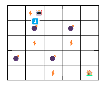
Let’s see an example how Q-learning can be used in a game wheere a robot reach to the end point through a maze.
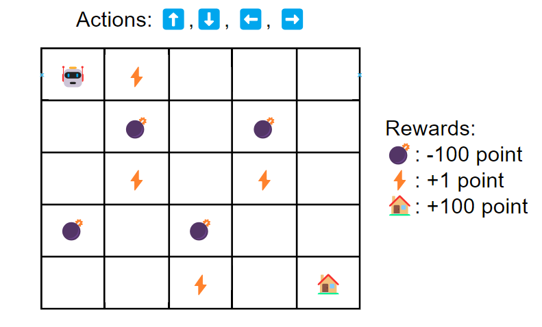
As you see in the above image, we have components of environment for the agents, which are state (5x5 grid), action, and reward. Our goal is to find the best action that maximize total reward. We are not likely find the best action in just one game. We might need to run multiple round of games. A game or trial is called episode in reinforcement learning.
In Q-learning, we update the value \(Q(s,a) \in \mathbb{R}^{25, 4}\). Bascially, \(Q\) is a 2D matrix where a row represetns a state and a column represents an action. It’s often called Q-table. The initial Q-table is a matrix filled with zeros.
| State | ⬆️ (1) | ⬇️ (2) | ⬅️ (3) | ➡️ (4) |
|---|---|---|---|---|
| 0 | 0 | 0 | 0 | 0 |
| 1 | 0 | 0 | 0 | 0 |
| 2 | 0 | 0 | 0 | 0 |
| 3 | 0 | 0 | 0 | 0 |
| 4 | 0 | 0 | 0 | 0 |
| ⋮ | ⋮ | ⋮ | ⋮ | ⋮ |
| 24 | 0 | 0 | 0 | 0 |
The initialized Q-table is persistent across episodes. When an episode ends, we keep all the Q-value updates. The next episode starts with the updated Q-table, so the agent has a slightly better idea of what actions are good or bad.
Let’s see the first episode setting learning rate \(\alpha = 0.5\) and discount factor \(\gamma = 0.9\).
1st Episode, Step 1:
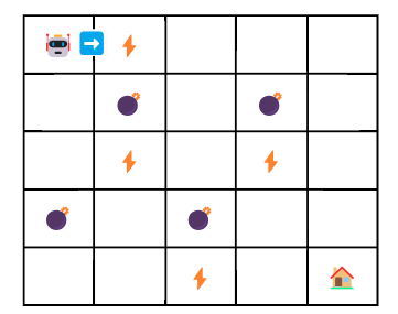
- current state: \(s_t=0\) (0,0)
- next state: \(s_{t+1}=1\)
- action: ➡️ (3)
- reward: \(r=+1\) \[ y_t = r_{t+1} + \gamma \max_{a'} Q(s_{t+1}, a') \] \[ y_t = 1 + 0.9 \max(1,a') \]
How do we know \(\max(1,a')\)? Simple. We can just look up the second row of Q-table.
| State | ⬆️ (0) | ⬇️ (1) | ⬅️ (2) | ➡️ (3) |
|---|---|---|---|---|
| 0 | 0 | 0 | 0 | 0 |
| 1 | 0 | 0 | 0 | 0 |
You see all actions are weighted at 0. Therefore, \(\max(1,a') = 0\). The the update will be given by:
\[ Q(0,3) \leftarrow Q(0,3) + \alpha[y_t - Q(s_t,a_t)] = 0.5 \]1st Episode, Step 2:
- current state: \(s_t=1\) (0,1)
- next state: \(s_{t+1}=6\) (1,1)
- action: ⬇️ (1)
- reward: \(r=-100\)
- update: \[ Q(1,1) \leftarrow Q(1,1) + \alpha[y_t - Q(1,1)] = 0 + 0.5[(-100+0.9\times0) -0] = -50 \]
In this setup, because hitting a 💣 is treated as a terminal state (big penalty, game over), the episode ends immediately after Step 2. Therefore, Q-table after the first episode will be:
| state | ⬆️ | ⬇️ | ⬅️ | ➡️ |
|---|---|---|---|---|
| 0 | 0 | 0 | 0 | 0.5 |
| 1 | 0 | -50 | 0 | 0 |
| others | 0 | 0 | 0 | 0 |
2nd Episode, Step 1
In the previous episode, the action was selected randomly because the initial Q-table is zeros. As the first and second entries are updated, will select actions according to the policy \(\pi^*(s) = \arg\max_{a} Q^*(s, a)\).
We want to know \(\pi^*(0)\) to pick an action. In the updated Q-table, the first entry (state 0) is [0, 0, 0, 0.5]. By using argmax, we know that ➡️ is the best action.
- action: ➡️ (3)
- current state: \(s_t=0\) (0,0)
- next state: \(s_{t+1}=1\)
- reward: \(r=+1\)
- update: \[ Q(0,3) \leftarrow 0.5 + 0.5[1 +0.9 \times 0 - 0.5] = 0.75 \]
5. Deep Q-Learning
Q-learning may work in a small environment. However, when the state–action space is very large, a tabular Q-table becomes computationally and memory intractable. In the previous section, we had a robot example. Let’s complicate it. Suppose the robot can now move in four diagonal directions (↗️, ↘️, ↙️, ↖️) in addition to the original four moves. We also scale the grid from \(5 \times 5\) to \(1,000 \times 1,000\). The Q-table size will be \(1,000,000 \times 8\).
There are even more complicated problems, such as Atari Breakout. In this game, the agent observes the entire screen image (210 × 160 pixels with 3 color channels) as the state, and must choose actions like “move left,” “move right,” or “fire.” This is a high-dimensional problem because each state is represented by tens of thousands of pixel values, and the number of possible screen configurations is astronomically large. We need a new solution beyond tabular Q-learning.
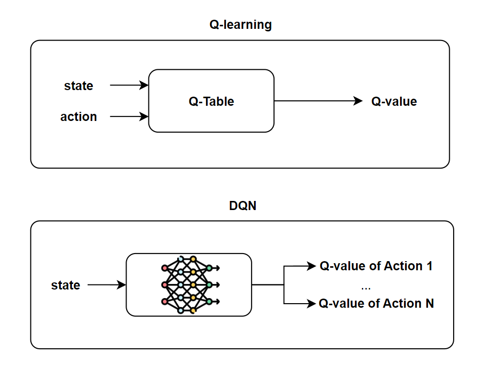
What if we can approximate Q-table, in other word optimal Q function (\(Q^*(s,a)\)). Deep Q-Learning (DQN) is a method that does exactly this. Instead of maintaining a huge Q-table, we use a neural network to approximate the Q-function:
\[ Q(s,a; \theta) \approx Q^*(s,a) \]Here, \(\theta\) represents the parameters (weights) of the neural network. Notice that in DQN, the network takes only the state \(s\) as input, hoping action \(a\) is implicityly learned by optimizing its corresponding output Q-value during training. (see the image at top of this blog.) The agent can generalize knowledge across similar states — something tabular Q-learning cannot do.
Deep Q-learning is trained by minimizing the Bellman error:
\[ \delta_t = y_t - Q(s_t, a_t) = r_{t+1} + \gamma \max_{a'} Q(s_{t+1}, a') - Q(s_t, a_t) \]We learned Bellamn error at section 4. But this is based on tabular Q-learning. As we move forward to DQN, we should introduce \(\theta\) to the Bellman error.
\[ \delta_t = r_{t+1} + \gamma \max_{a'} Q(s_{t+1}, a'; \theta^-) - Q(s_t, a_t; \theta) \]\(\max_{a'} Q(s_{t+1}, a'; \theta^-)\) denotes a value of the best action in the next state, computed with the target network \(\theta^-\) for stability. \(Q(s_t, a_t; \theta)\) is a current estimate from a online network \(\theta\).
Wait a second. What’s the difference between the target network \(\theta^-\) and online network \(\theta\)? Are we using two networks? Kind of. Basically, only \(\theta\) is updated via training. \(\theta^-\) is a lagged copy of \(\theta\). At the beginning, we initialize both networks identically (i.e., \(\theta^- \leftarrow \theta\)). During training, we keep updating \(\theta\) with gradient descent at every step, but \(\theta^-\) stays frozen. After some fixed interval (say every 1000 updates), we copy the current parameters of the online network into the target network (\(\theta \leftarrow \theta\)).
But why do we need the target network \(\theta^-\) in the first place? The answer is to stabilize the learning process. If we didn’t have a target network, the loss function would look like this:
\[ \mathcal{L}(\theta) = \left( r + \gamma \max_{a'} Q(s_{t+1}, a'; \theta) - Q(s_t, a_t; \theta) \right)^2 \]Here both the prediction and the target come from the same network \(\theta\). I couldn’t intuitively think this causes unstablized learning. The target network was first introduced by Human-level control through deep reinforcement learning (Mnih et al., 2015). The authors emperically demonstrated that a DQN underperformed when training a network without a target network. You can refer to Table 3 from the paper. See what the authors said about it.
The second modification to online Q-learning aimed at further improving the stability of our method with neural networks is to use a separate network for generating the targets \(y_j\) in the Q-learning update. More precisely, every \(C\) updates we clone the network \(Q\) to obtain a target network \(\hat{Q}\) and use \(\hat{Q}\) for generating the Q-learning targets \(y_j\) for the following \(C\) updates to \(Q\). This modification makes the algorithm more stable compared to standard online Q-learning, where an update that increases \(Q(s_t, a_t)\) often also increases \(Q(s_{t+1}, a)\) for all \(a\) and hence also increases the target \(y_j\), possibly leading to oscillations or divergence of the policy.
So now we are convinced why the target network is needed. So the ideal loss function would be:
\[ \mathcal{L}(\theta) = \left( r + \gamma \max_{a'} Q(s_{t+1}, a'; \theta^-) - Q(s_t, a_t; \theta) \right)^2 \].
The theoretical form that the authors expressed is:
\[ \mathcal{L}(\theta) = \mathbb{E}_{(s_t, a_t, r, s_{t+1}) \sim U(D)} \left[ \Big( r + \gamma \max_{a'} Q(s_{t+1}, a'; \theta^-) - Q(s_t, a_t; \theta) \Big)^2 \right] \]where \(U(D)\) is a uniform distribution. In practice, this expectation is approximated by sampling mini-batches from the replay buffer rather than computing over the entire distribution. Together with the target network, this design makes Deep Q-Learning both scalable to high-dimensional environments and significantly more stable than naive neural-network Q-learning.
Conclusion
Reinforcement learning is not easy to grasp. It requires some background in probability, dynamic programming, and optimization. That is why we started from the ground up: beginning with the Markov property, extending it into Markov Decision Processes (MDPs), and then introducing the value function and Q-learning. This journey from Markov chains to DQN shows how reinforcement learning evolved from simple mathematical foundations to powerful deep learning–based methods that can solve complex, high-dimensional problems.