 In this blog post, I will share my journey with my final project for my computer graphics course at school. Computer graphics is used to generate images, animations, and visual effects. You might see mechanical engineering students doing CAD (Computer-Aided Design) work — that’s also a form of computer graphics, though it focuses more on precision modeling and simulation for physical systems. OpenGL is is an API for rendering 2D and 3D vector graphics, commonly used by engineers and architects for CAD behind the hood. For my project, I implemented a basic 3D SPH system using OpenGL for real-time visualization. The simulation space is a cube filled with particles that respond to forces like pressure, viscosity, and external gravity. Each frame, the particle positions are updated based on SPH equations, and OpenGL renders the updated state, giving a dynamic and continuous fluid effect. However, SPH simulation is computationally expensive because it considers interactions between particles in a nested manner. I optimized the simulation using Compute Unified Device Architecture (CUDA). CUDA is an API developed by NVIDIA that is used for parallel computation on GPUs. I observed 98% performance improvement by adopting CUDA. Check my Github Repository for the code.
SPH Simulation Workflow
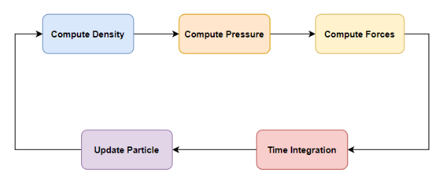 SPH is a particle-based method for simulating fluid dynamics by modeling fluids as discrete particles that carry properties like mass, velocity, and pressure. The simulation begins by computing the density at each particle based on its proximity to neighboring particles. Using the density, pressure is then calculated to capture how particles push against one another. These pressure values, along with other physical influences like viscosity and gravity, are used to compute forces acting on each particle. Finally, the simulation performs time integration to update particle velocities and positions, repeating this cycle continuously to simulate realistic fluid motion. Each particle in the SPH simulation carries five key attributes:
- Position – the particle’s location in 3D space.
- Velocity – the speed and direction of the particle’s movement.
- Force – the net force acting on the particle, derived from pressure, viscosity, and external influences like gravity.
- Density – a measure of how much mass surrounds the particle, computed from nearby particles.
- Pressure – the internal pressure at the particle’s location, calculated from its density and used to simulate fluid behavior.
Mathmatical background
Algorithm
- Create particles arranged evenly in a 3D grid
- Find \(\mathcal{N}(p_i)\) neighbors of each particle
- for each \(p_i\) in \(P\) do
- for each \(\mathcal{n_j}(p_i)\) in \(\mathcal{N}(p_i)\)
- Accumulate density
- Compute pressure using density
- Initialize total force \(f_i=0\)
- for each \(\mathcal{n_j}(p_i)\) in \(\mathcal{N}(p_i)\)
- Accumulate pressure force into \(f_i\)
- Accumulate viscosity force into \(f_i\)
- Add gravity force to \(f_i\)
- for each \(\mathcal{n_j}(p_i)\) in \(\mathcal{N}(p_i)\)
- for each \(p_i\) in \(P\) do
- update velocity
- update position
- collision handling
- repeat 2 to 4
Density Computation
The density \(\rho_i\) at particle \(i\) is computed by summing contributions from neighboring particles \(j\):
\[ \rho_i = \sum_j m_j W_{poly6}(r_{ij},h) \]- \(m_j\): mass of particle \(j\)
- \(r_{ij}\): distance between particles \(i\) and \(j\)
- \(h\): smoothing radius
- \(W_{poly6}\) kernel smoothing function \[ W_{\text{poly6}}(r, h) = \begin{cases} \dfrac{315}{64 \pi h^9}(h^2 - r^2)^3, & r \leq h \\ 0, & r > h \end{cases} \]
Pressure Computation (Equation of State)
The pressure \(p_i\) at particle \(i\) is determined from the density deviation using an equation of state:
\[p_i = k(\rho_i - \rho_0)\]- \(k\): Gas constant
- \(\rho_0\): rest density
Momentum Equation (Navier-Stokes Forces)
For particle \( i \), the total force \( \mathbf{F}_i \) includes pressure, viscosity, and gravity:
\[ \mathbf{F}_i = \mathbf{F}_i^{\text{pressure}} + \mathbf{F}_i^{\text{viscosity}} + \mathbf{F}_i^{\text{gravity}} \]- \(\mathbf{F}_i^{\text{pressure}} = -\sum_{j \ne i} m \frac{p_i + p_j}{2\rho_j} \nabla W_{\text{spiky}}(\mathbf{r}_{ij}, h)\)
- \(m\): mass of particle \(j\)
- \(p\): pressure of a particle
- \(\nabla W_{\text{spiky}}\): Spiky Gradient \[ \nabla W_{\text{spiky}}(\mathbf{r}, h) = \begin{cases} -\dfrac{45}{\pi h^6}(h - r)^2 \dfrac{r_{ij}}{r}, & 0 < r \leq h \\ 0, & \text{otherwise} \end{cases} \]
- \(\mathbf{F}_i^{\text{viscosity}} = \sum_{j \ne i} \mu m_j \frac{\mathbf{v}_j - \mathbf{v}_i}{\rho_j} \nabla^2 W_{\text{viscosity}}(\mathbf{r}_{ij}, h)\)
- \(\mu\): viscosity coefficient
- \(v\): velocity
- Viscosity Laplacian \( \nabla^2 W_{\text{viscosity}}\) \[ \nabla^2 W_{\text{viscosity}}(r, h) = \begin{cases} \dfrac{45}{\pi h^6}(h - r), & r \leq h \\ 0, & r > h \end{cases} \]
- \(\mathbf{F}_i^{\text{gravity}} = \rho_i \mathbf{g}\)
- \(g\): gravitational acceleration vector
- \(\rho\): density
Time Integration (Semi-implicit Euler)
- Acceleration \(a_i = \dfrac{F_i}{\rho_i}\)
- Velocity Update: \(\mathbf{v}^{new}_i = \mathbf{v}^{old}_i + a_i \Delta t\)
- Position Update: \(\mathbf{x}^{new}_i = \mathbf{x}^{old}_i + \mathbf{v}^{new}_i \Delta t\)
Collision Damping at Boundary
If a particle hits a boundary, its velocity is modified to prevent it from escaping the simulation domain. Specifically, the velocity is scaled by a damping factor:
\[\mathbf{v}^{new} = \mathbf{v}^{old} \times d\]- \(\mathbf{v}\): velocity of a particle
- \(d\): damping factor
Predefined Parameters for SPH simulation
- \(k\): gas constant
- \(\rho_0\): rest density
- \(m\): mass of particle
- \(\mu\): viscosity coefficient
- \(g\): gravity
- \(\Delta t\): time step
- \(h\): smoothing radius
- \(d\): damping factor at collision
Overshooting particles with a perfect symmetry
In this section, we will see problems I first encountered when I asked chatgpt for the baseline simulation. Let’s take a look at the part of SPHSystem.cpp.
// SPHParameters.h
const float TIME_STEP = 0.005f;
const float MASS = 10.0f; // kg
const float SMOOTHING_RADIUS = 0.045f;
const float GRAVITY = -9.81f;
const float DAMPING = -0.3f;

// SPHSystem.cpp
void SPHSystem::initializeParticles() {
    for (int x = 0; x < numX; ++x) {
        for (int y = 0; y < numY; ++y) {
            for (int z = 0; z < numZ; ++z) {
                glm::vec3 pos = glm::vec3(
                    x * spacing,
                    y * spacing + 0.5f,
                    z * spacing
                );
                particles.emplace_back(pos);
            }
        }
    }
}

void SPHSystem::integrate() {
    //Defines the simulation bounding box: all particles must stay within [0, 1] along x, y, and z
    const glm::vec3 boundsMin(0.0f, 0.0f, 0.0f);
    const glm::vec3 boundsMax(1.0f, 1.0f, 1.0f);

    for (auto& p : particles) {
        // Acceleration
        glm::vec3 acceleration = p.force / p.density;

        //Semi-implicit Euler
        p.velocity += acceleration * TIME_STEP; // velocity update
        p.position += p.velocity * TIME_STEP; // position update

        // Simple boundary constraint that particles stay within a defined simulation box
        for (int i = 0; i < 3; ++i) {
            if (p.position[i] < boundsMin[i]) {
                p.position[i] = boundsMin[i];
                p.velocity[i] *= DAMPING;
            } else if (p.position[i] > boundsMax[i]) {
                p.position[i] = boundsMax[i];
                p.velocity[i] *= DAMPING;
            }
        }
    }
}
The initializeParticles function creates a 3D grid of particles arranged in a cubic grid structure. The cubic particles are located 0.5f high and start falling in the begining of simulation due to the gravity pull. When particles hit the bottom, they bounce upward with lower velocity. The below animation is rendered simulation.
The movements of particles were not I expected. Why particles oscillate without losing energy? This problem is called overshooting. Large updates to position and velocity can overshoot expected particle motion. Then, what parameter should we tweak to address overshooting? Time step \(\Delta t\). Let’s lower the TIME_STEP to 0.0008 and run the simulating.
Now we see the particles lose energy over time. But why it still doesn’t look like fluid? We need to break perfect symmetry. When particles are initialized in a perfectly uniform grid, they behave in unnaturally synchronized ways. Every particle experiences nearly identical forces from its neighbors. To make our simulation more physically plausible, we can introduce a small amount of random noise to the initial positions of particles.
void SPHSystem::initializeParticles() {
    std::srand(static_cast<unsigned>(std::time(nullptr))); // Optional: seed RNG once

    float noiseScale = spacing * 0.1f; // 10% of spacing

    for (int x = 0; x < numX; ++x) {
        for (int y = 0; y < numY; ++y) {
            for (int z = 0; z < numZ; ++z) {
                float nx = ((std::rand() % 1000) / 1000.0f - 0.5f) * noiseScale;
                float ny = ((std::rand() % 1000) / 1000.0f - 0.5f) * noiseScale;
                float nz = ((std::rand() % 1000) / 1000.0f - 0.5f) * noiseScale;

                glm::vec3 pos = glm::vec3(
                    x * spacing + nx,
                    y * spacing + 0.5f + ny,
                    z * spacing + nz
                );
                particles.emplace_back(pos);
            }
        }
    }
}
Unpredictable movements of particles make the simulation look more natural and fluid-like.
Basic of CUDA
It’s well known that multi-processing can optimize a program using parallization. Each core computes a separate chunk of the workload simultaneously, reducing overall execution time. If you have an fancy CPU, it might have 16 cores. This is nothing compared to GPUs. My GPU, RTX 3060 Ti, has has 4,864 CUDA cores. No matter what language you used, when your computer compiles your program, it will eventually translate it into assembly instructions. To run GPU-based program, it needs to be translated into an architecture that the NVIDIA GPU understands. The architecture is called CUDA (Compute Unified Device Architecture).
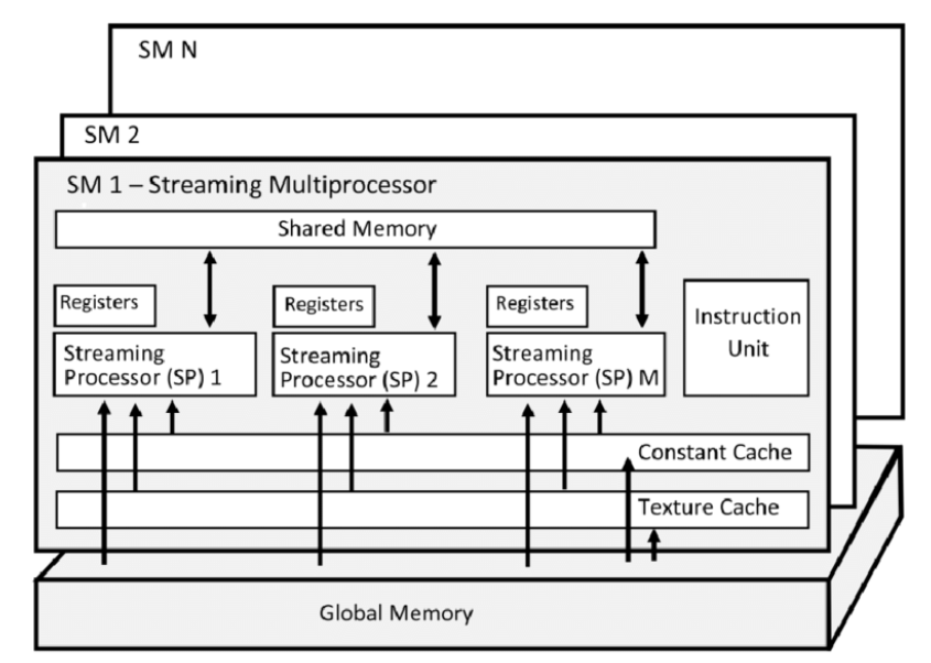
CUDA consists of multiple streaming multiprocessors (SMs) bridged by global memory. Through the global memory, SM shares the resource. In each SM, there are multiple streaming processors (SPs) bridged by shared memory. A single thread is processed by SP. A group of thread is called a thread block, which is processed by SM. A kernel grid is the collection of thread blocks that are launched to execute a kernel function on the GPU.
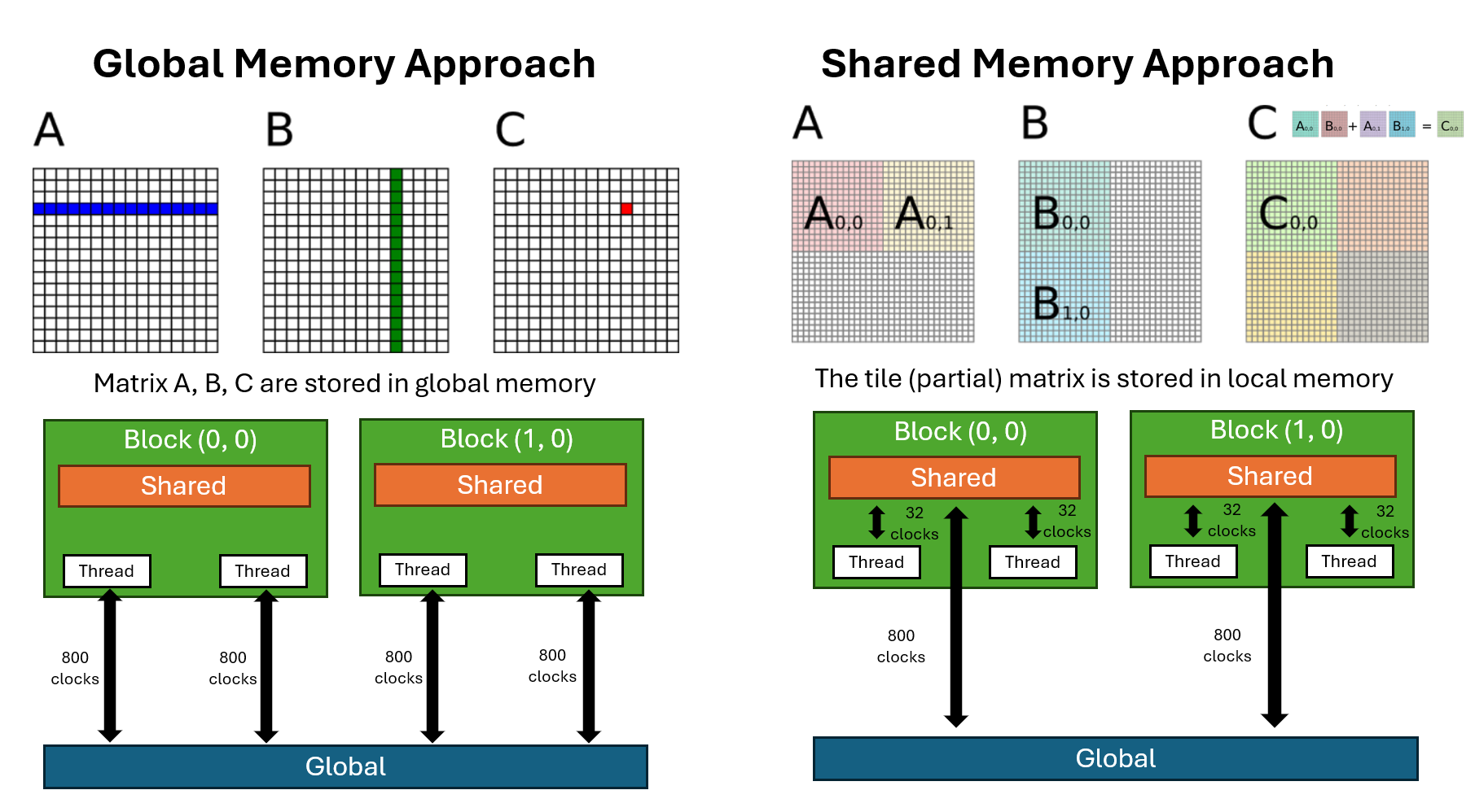
The simiplest CUDA-parallization approach would be using global memory. However, it can be further opimized if you use shared memory. Shared memory has much lower latency and higher bandwidth compared to global memory. Of course, there is trade-off. Shared memory has much less capacity. This means you have to divide your data into smaller chunks and carefully load only the necessary portions into shared memory.
The below image compares global memory and shared memory approaches for matrix multiplication in CUDA. The shared memory appraoch is also called a tiling technique, which divide data into smaller chunk.
Optimize SPH Algorithm using CUDA
In this section, we will optimize the SPH algorithm using CUDA global functions. Let’s take a look at SPHSystem.h to see scaffold of the data structure.
class SPHSystem {
public:
    std::vector<Particle> particles;

    SPHSystem();
    ~SPHSystem();

    void computeDensityPressure();
    void computeForces();
    void integrate();

private:
    void initializeParticles();
};
The first step we will optimize the computeDensityPressure function. When launching a global kernel in CUDA, you must specify number of blocks and number of threads per block besides the arguments. kernel<<<numBlocks, threadsPerBlock>>>();. There is a folmula for number of blocks given the size of your data. int blocks = (size + threadsPerBlock - 1) / threadsPerBlock; In our case, the size is the number of particles.
inline dim3 gridFor(int N,int block){ return dim3((N+block-1)/block); }

void SPHSystemCUDA::computeDensityPressure(){
    densityPressureKernel<<<gridFor(N_,256),256>>>(N_,d_pos_,d_density_,d_pressure_);
    cudaDeviceSynchronize();
}
The computeDensityPressure function will call global kernel densityPressureKernel. In addition to the global function, I provide CPU-based function for comparison. First thing we notice is densityPressureKernel takes arguments while CPU-based function doesn’t. Second, the global kernel is O(n) while the other one is O(n^2). I first answer the second question. Let’s say we have 100 particles. In the CPU-based function, the program iterates over each particle sequentially. In the CUDA global version, each thread is responsible for handling a single particle, identified by its thread id. Now let’s answer the first question.
In global kernel, we cannot access particle directly because CUDA only supports low-level C++ objects like float or float3. So we need containers for particle.position, particle.density, and particle.pressure. The three array arguments, pos, dens, and pres are stored in global memory, where all threads can access them.
__global__ void densityPressureKernel(
        int N, const float3* pos, float* dens, float* pres)
{
    int id = blockIdx.x*blockDim.x + threadIdx.x;
    if (id>=N) return;

    float density = 0.f;
    float3 pi = pos[id];

    for (int j=0; j<N; ++j) {
        float3 rij{
            pos[j].x - pi.x,
            pos[j].y - pi.y,
            pos[j].z - pi.z};
        float r2 = rij.x*rij.x + rij.y*rij.y + rij.z*rij.z;
        density += MASS * poly6Kernel(r2, SMOOTHING_RADIUS);
    }
    dens[id] = density;
    pres[id] = GAS_CONSTANT * (density - REST_DENSITY);
}
//    ↑ GPU-based function
//    │
//    │
//    │
//    ↓ CPU-based function
void SPHSystem::computeDensityPressure() {
    for (auto& pi : particles) {
        pi.density = 0.0f;
        for (const auto& pj : particles) {
            glm::vec3 rij = pj.position - pi.position;
            float r2 = glm::dot(rij, rij);
            pi.density += MASS * poly6Kernel(r2, SMOOTHING_RADIUS);
        }
        pi.pressure = GAS_CONSTANT * (pi.density - REST_DENSITY);
    }
}
We are gonna skip computeForces function and jump to integrate function. We see CUDA function cudaMemcpy. In CUDA code, if variable starts with h like h_pos, it means that the data resides on host (CPU). If variable starts with d, it means the data is on device (GPU). In the below code, cudaMemcpy moves data from host to device. Lastly, we update particles with h_pos transfered from GPU to CPU.
void SPHSystemCUDA::integrate(){
    integrateKernel<<<gridFor(N_,256),256>>>(N_,d_pos_,d_vel_,d_force_,d_density_);
    cudaDeviceSynchronize();

    // copy positions back so ParticleRenderer can update VBO
    std::vector<float3> h_pos(N_);
    cudaMemcpy(h_pos.data(), d_pos_, N_*sizeof(float3), cudaMemcpyDeviceToHost);

    for (int i=0;i<N_;++i){
        particles[i].position = glm::vec3(h_pos[i].x,h_pos[i].y,h_pos[i].z);
    }
}
Check my code for details about the CUDA script. You can see how fast the CUDA SPH simulation runs.
| Approach | # Particles | Total Time (sec) |
|---|---|---|
| CPU | 125 | 4.161 |
| CUDA | 125 | 1.471 |
| CPU | 1,000 | 169.067 |
| CUDA | 1,000 | 1.742 |