 Most large language models (LLMs) today are autoregressive models. Before LLMs, NLP was fragmented — different problems like text classification, translation, summarization, and question answering all needed their own models, datasets, and training tricks. But then came GPT-2, and everything changed. GPT-2 is an autoregressive model trained purely on text generation — predicting the next word in a sequence — that’s called decoding.Surprisingly, this simple setup made it capable of handling a wide range of NLP tasks, often without fine-tuning. Once you can generate text well, solving other NLP problems becomes almost trivial. You might’ve heard terms like temperature, top-k, and top-p, which are parameters for LLM inference. In this blog post, we’ll explore how the model chooses from possible next words, how randomness is controlled, and what happens under the hood when you ask an LLM to generate text.
Autoregressive Model
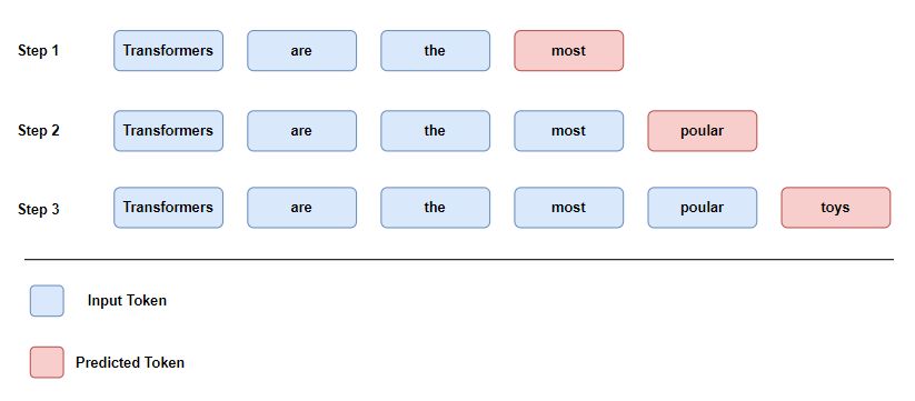
An autoregressive model generates one token at a time, each conditioned on the tokens it has already generated. In other words, it builds sequences step by step, always looking at the past to predict the future. At its core, it’s a way to model time series data. Before the rise of Transformers, architectures like RNNs, LSTMs, and GRUs were the go-to choices for building autoregressive models. But today, especially in the context of large language models, decoder-only Transformers have taken over. In this blog, we’ll focus on how these modern autoregressive models are used for text generation.
Mathematical Formulation of Text Generation
In autoregressive models, the goal is to find the most likely output sequence given the input. We can start estimating the conditional probability of a target sequence \( \mathbf{y} = (y_1, y_2, \ldots, y_N) \) given some input \( \mathbf{x} \). This could be a prompt, a source sentence (in translation), or even empty input (as in pure language modeling).
The core idea is to decompose the joint probability of the output sequence into a product of conditional probabilities:
\[ P(y_1, y_2, \ldots, y_N \mid \mathbf{x}) = \prod_{t=1}^{N} P(y_t \mid y_1, \ldots, y_{t-1}, \mathbf{x}) \]Or more compactly:
\[ P(\mathbf{y} \mid \mathbf{x}) = \prod_{t=1}^{N} P(y_t \mid y_{< t}, \mathbf{x}) \]Here, \( y_{< t} \) refers to all previous tokens before time step \( t \).
At each step, the language model scores all possible next words and assigns a number to each one — these are called logits \( z_{t,i} \). For each token \( w_i \) in the vocabulary at step \( t \), we can obtain the probability distribution over the next possible token by applying the softmax function:
\[ P(y_t = w_i \mid y_{< t}, \mathbf{x}) = \text{softmax}(z_{t,i}) \]The goal of most decoding methods is to search for the most likely overall sequence by selecting a \( \hat{\mathbf{y}} \) that maximizes the conditional probability:
\[ \hat{\mathbf{y}} = \arg\max_{\mathbf{y}} P(\mathbf{y} \mid \mathbf{x}) \]However, we have a problem. Finding \( \hat{\mathbf{y}} \) exactly would require evaluating all possible sequences, which is computationally infeasible due to the combinatorial explosion of possibilities. Think about how many tokens we are dealing with. In GPT-2, the vocabulary size is around 50,000 tokens, and generating even a moderately long sequence—say, 20 tokens—would involve evaluating \(50,000^{20}\) possible combinations.
This exponential growth makes exact search intractable. So we have to rely on approximation instead to generate output sequences. There are two main approches:
- Deterministic method, which deterministically selects tokens based on model confidence (e.g., greedy decoding, beam search)
- Stochastic method, which introduces randomness to explore multiple plausible continuations (e.g., top-k, top-p)
Deterministic Methods - Greedy Search Decoding
Greedy decoding is the simplest decoding strategy. At each timestep, the model selects the token with the highest probability — the one it’s most confident about — and adds it to the output sequence.
Formally, at each time step \( t \), the next token \( y_t \) is selected as:
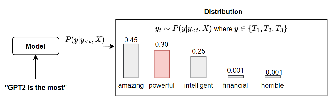
\[ y_t = \arg\max_{w_i} P(y_t = w_i \mid y_{< t}, \mathbf{x}) \]This process continues until the model generates an end-of-sequence token (i.e. <eos>) or reaches a maximum length. While greedy decoding is fast and easy to implement, it has significant limitations. Because it always picks the most likely next token, it can get stuck in repetitive output sequences. For example, let’s say you are given with the following prompt.
GPT2 are the most
The most likely next word would probably be a positive adjective like amazing, miraculous, or powerful. Let’s say the model picks “amazing”:
GPT2 are the most amazing
Now let’s think about what might come next. If you look up “amazing” in a dictionary, you’ll find synonyms like fantastic and incredible. In a greedy decoding setup, the model might keep choosing the next most probable word — which could just be another synonym. That’s how you end up with repetitive outputs like:
GPT2 are the most amazing fantastic powerful
This happens because greedy decoding favors locally optimal choices at every step, without regard for sentence structure, coherence, or redundancy over the full sequence.
Deterministic Methods - Beam Search Decoding
 ref. Decoding Methods for Generative AI
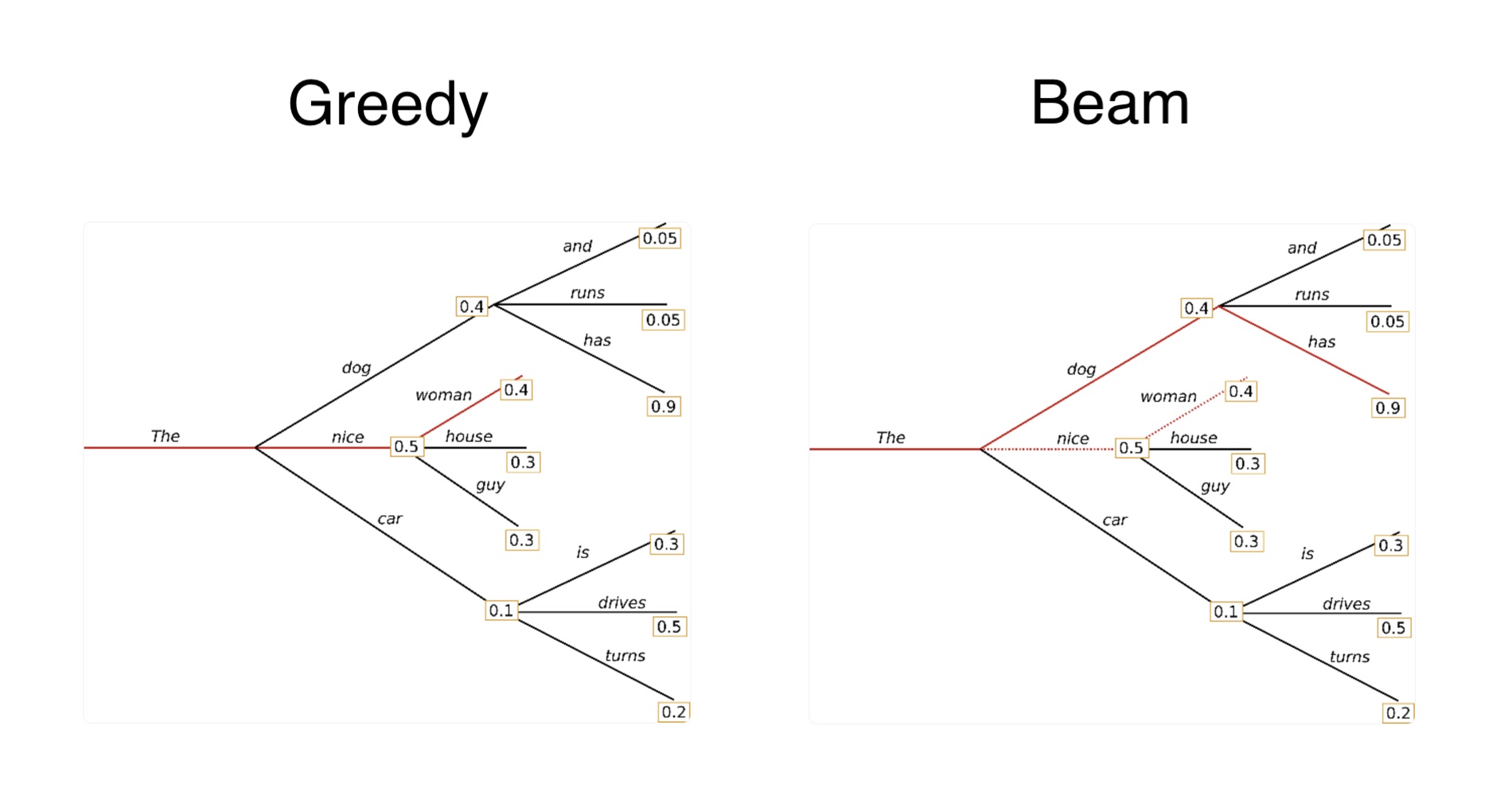
Beam search decoding addresses a key limitation of greedy decoding: its tendency to get stuck in local optima by always picking the most probable token at each step.
Instead of choosing just one token at each timestep, beam search keeps track of the top \( k \) most probable partial sequences — known as the beam width. At each step, it expands each of these sequences by all possible next tokens, then keeps the top \( k \) new sequences based on their cumulative probabilities.
This allows the model to explore multiple potential continuations in parallel, rather than committing to a single path too early. By the end, it selects the complete sequence with the highest overall probability.
However, beam search is not completely free from repetitive sequence because it is still based on maximizing likelihood. Even if we have a very large \(k\), the algorithm may still favor sequences composed of high-probability tokens, which often include repeated words or phrases. The model might be confident for output sequences, but that may lack diversity or creativity.
In other words, beam search may underperform in open-ended text. For example, when generating a creative story or a conversational response, it often produces bland, repetitive, or overly generic outputs. Suppose a user prompts a model with, “Tell me a story about a robot who learns to paint.” Beam search might yield:
There was a robot. The robot wanted to paint. The robot learned to paint. The robot became a great painter.
This is coherent and grammatically correct, but it’s also dull and predictable. Even increasing the beam width doesn’t help much — it may just produce multiple variations of the same generic idea. To address this lack of diversity, sampling methods are employed to introduce randomness
Before we dive into sampling methods, it’s important to understand a key trade-off in text generation: coherence vs. diversity.
- If we always choose the most likely next word (as in greedy or beam search), we get coherent but often dull and repetitive text.
- If we allow more randomness, we can generate more diverse and creative outputs — but at the risk of losing coherence or producing nonsensical sentences.
Stochastic Methods - Top-k Sampling Decoding
 Instead of selecting the single most likely token, top-k sampling restricts the candidate pool to the top \( k \) tokens with the highest probabilities. Then, it randomly samples from that pool while low-probability tokens are completely ignored.
What we expect from the degree of \(k\)?
- Small \( k \) (e.g., 3): More coherent but less diverse.
- Large \( k \) (e.g., 50): More diverse but with increased risk of incoherence.
Stochastice Methods - Top-p Sampling Decoding
The top-p sampling, also called nucleus samplling, , is a more adaptive alternative to top-k sampling. Instead of selecting a fixed number of top tokens, top-p sampling chooses from the smallest possible set of tokens whose cumulative probability exceeds a threshold \( p \). This is how it works:
- Sort all vocabulary tokens by their predicted probability in descending order.
- Starting from the top, include tokens in the candidate pool until their combined probability exceeds \( p \) (e.g., 0.9).
- Sample the next token from this dynamically sized set.
This means the number of candidate tokens changes depending on the shape of the probability distribution. If the model is confident, the set might be very small; if it’s uncertain, the set might include more options.
I have a question for you. Can \(p\) exceed 1? The answer is no. Because we already applied softmax to the logits \(z_{t, i}\), the cumulative cumulative probability always add up to 1.
Okay so when should we consider using top-p sampling over top-k sampling? Top-p sampling is more flexible than top-k:
- When the model is very confident (probability mass is concentrated), top-p behaves like greedy decoding.
- When the model is unsure (probability mass is more spread out), top-p allows more exploration.
This adaptiveness helps balance fluency and diversity better than top-k in many cases.
Stochastice Methods - Temperature
 Temperature controls the randomness of the model’s predictions during sampling. However, temperature is not a sampling method on its own. Temperature is a modifier that adjusts the shape of the probability distribution before sampling happens — whether you’re using top-k or top-p.
By default, a language model produces a probability distribution over the vocabulary using softmax. Temperature modifies the shape of this distribution before sampling. Mathematically, logits \( z_i \) are divided by a temperature value \( T \) before applying softmax:
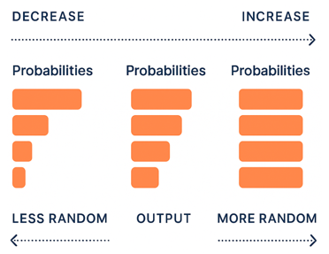
\[ P(y_t = w_i) = \frac{\exp(z_i / T)}{\sum_j \exp(z_j / T)} \]- Low temperature (< 1.0) sharpens the distribution:
- High-probability tokens become even more likely.
- Output is more deterministic and focused.
- High temperature (> 1.0) flattens the distribution:
- Differences between token probabilities shrink.
- Output becomes more diverse and creative — but riskier.
I have another question for you. Can we use temperature for greedy search or beam search? Well, there is no point of using temperature in this case. Both search algorithms will always choose the probable token anyway. The temperature can change the shape of the distribution, but it doesn’t change the relative ordering of token probabilities — so the top-1 token remains the same, regardless of the temperature.
Conclusion
Autoregressive language models generate text one token at a time, predicting the next word based on everything generated so far.
Greedy and beam search offer more deterministic but often result in repetitive or generic outputs. Sampling-based methods like top-k, top-p, and temperature introduce controlled randomness to improve diversity and creativity. By understanding these decoding strategies, you can better steer large language models toward the kind of output you want.
Reference
- https://dev.to/nareshnishad/gpt-2-and-gpt-3-the-evolution-of-language-models-15bh
- Natural Language Processing with Transformers; Lewis Tunstall et al.
- https://heidloff.net/article/greedy-beam-sampling/