From Policy Gradient to GRPO: Policy Optimization for LLM Training

You’ve probably heard that DeepSeek R1 was fine-tuned using reinforcement learning, specifically an algorithm called Generalized Reparameterized Policy Optimization (GRPO). DeepSeek research team demostrated that reinforcement learning (RL) without any supervised fine-tuning can teach LLMs to reason, and this drew widespread interest and scrutiny across academia. In my previous blog post, Mathmatical Foundation from Markov to Deep Q-learning, we dabbled in Q-learning, which is value-based (off-policy) RL where the agent learns value (\(Q\) or \(V\)) and derives its policy \(\pi\) from the value. GRPO, which is what we are gonna learn about in this post, is a policy-based RL where the agent directly learns the policy. We’re not going to jump straight into GRPO. Instead, we will walk through policy-based RL methods, starting with the policy gradient, actor-critic method, proximal policy optimization (PPO), and finally GRPO.

Policy Gradient

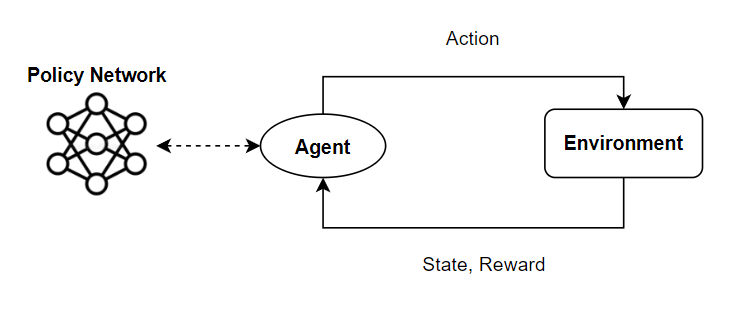
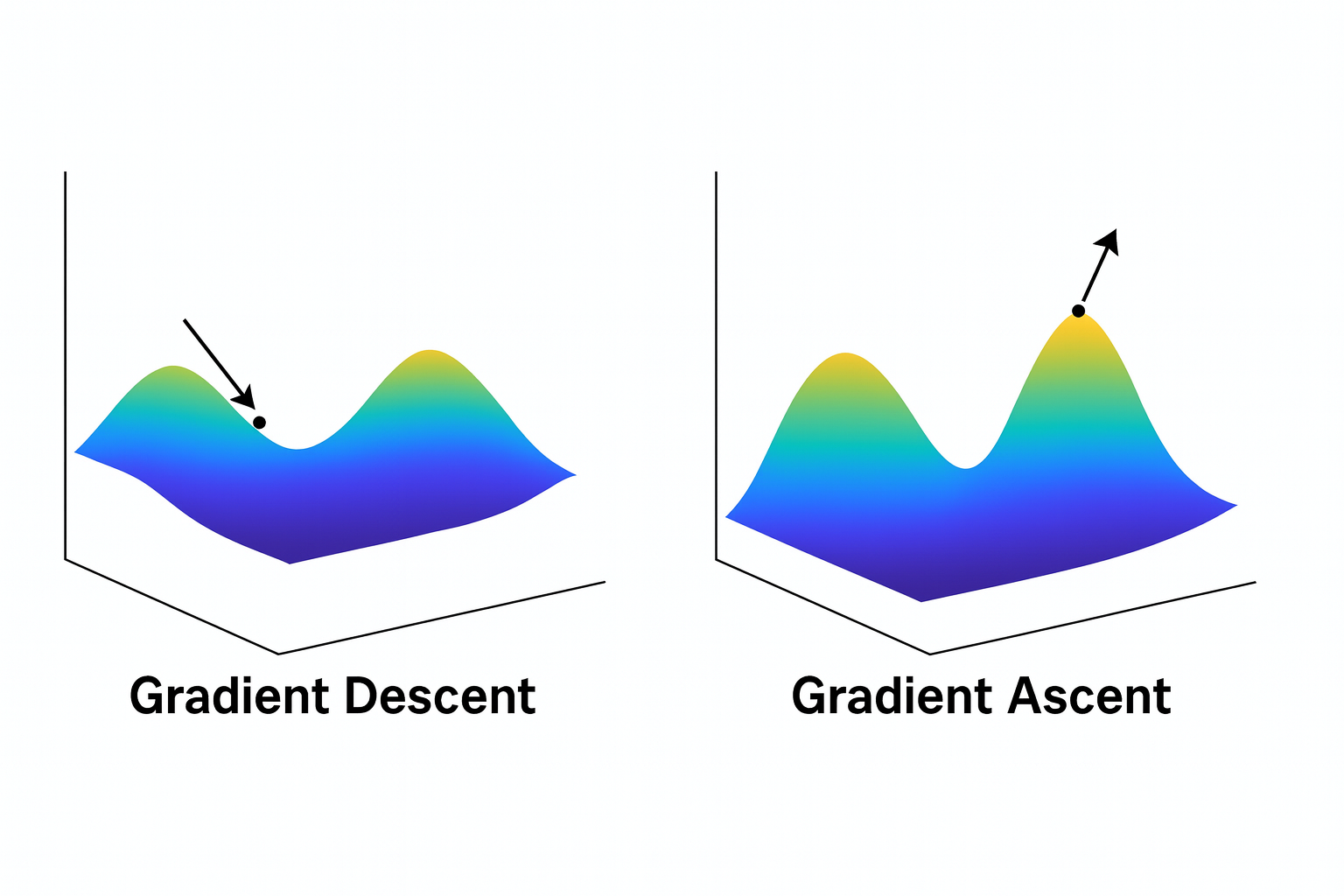
Before diving into PPO, you should definitely understand the policy gradient concept first. In my previous post, I didn’t cover the policy gradient because it was oriented to introduce Q-learning. Q-learning belongs to the value-based family of reinforcement learning, where the agent learns a value function \(Q(s,a)\) or \(V(s)\) and derives its policy. On the other hand, policy-based methods like PPO and GRPO take a different approach. Instead of learning values and deriving a policy from them, the agent directly learns the policy itself by obtimizing it through gradient ascent on the expected reward. Yes, I said gradient ascent, not gradient descent. In supervised learning, like classification or regression, we minimize a loss function (e.g., cross-entropy, MSE), which means we use the gradient descent to reduce an error.

Meanwhile, in reinforcement learning, we maximize expected cumulative reward:

\[ G_t = R_{t+1} + \gamma R_{t+2} + \gamma^2 R_{t+3} + \ldots = \sum_{k=0}^{\infty} \gamma^k R_{t+k+1} \\ J(\theta) = \mathbb E_{\pi\theta}[G_t] \quad (1) \]

Here, \(\theta\) represents the parameters of the policy network \(\pi_{\theta}\). At each training step, we udpate the network parameters using the gradient \(\nabla_{\theta}J(\theta)\) and a learning rate \(\alpha\) Mathematically, the update rule is defined as:

\[ \theta \leftarrow \theta + \alpha \nabla_{\theta}J(\theta) \]

Okay, we have an euqation for learning but we have a problem. \(J(\theta)\) does not seem to depend on the policy \(\pi_{\theta}\). If we don’t have expression with respect to \(\pi_{\theta}\), we cannot calculate its gradient because the network we are optimizing is the policy \(\pi_{\theta}\) itself. How can we rewrite \(\mathbb{E}_{\pi_\theta}[G_t]\) with respect to policy \(\pi_{\theta}\)? We will get there but first, let’s look into the definition of the expected value.

The expected value is a predicted value of a variable, calculated as the sum of all possible values each multiplied by the probability of its occurrence:

\[ \mathbb{E}[X] = \sum P(x_i) x_i = \int xP(x)dx \]

Here, \(X\) is a random variable with possible outcomes \(x\). But in RL context, what would be the variable? This is where we should know about state action trajectory. Based on a policy, an agent generates a sequence of states and action; i.e., trajectory:

\[ \tau : (s_0, a_0, s_1, a_1, \ldots, s_t, a_t) \]

In RL, a trajectory \(\tau\) is a random variable. We can expand the objective function \(J(\theta)\).

\[ J(\theta) = \mathbb{E}_{\pi_\theta}[G_t] = \int P_\theta(\tau) G(\tau) \]

The probability of observing that trajectory under policy \(\pi_\theta\) is:

\[ P_\theta(\tau) = P(s_0) \prod_{t=0}^{T-1} \pi_\theta(a_t|s_t)\, P(s_{t+1}|s_t,a_t) \]

Now, we see \(J(\theta)\) is dependent to the policy \(\pi_{\theta}\). However, this is not good form when using computer for calculation. Because product of probability, \(\prod P(x)\), can give you a very tiny number, which can cause underflow and numerical precision loss. That’s where the logarithm comes in since product rule turns into a sum.

\[ \nabla_{\theta} J(\theta) = \int \nabla_{\theta} P_\theta(\tau) G(\tau) \]

By applying log-derivative trick, \( \nabla_{\theta} P_\theta(\tau) = P_{\theta} (\tau) \nabla_{\theta} \log P_{\theta}(\tau)\),

\[ \nabla_{\theta} J(\theta) = \int P_\theta(\tau) \nabla_{\theta} \log P_\theta(\tau) G(\tau) \]

Since \(P_\theta(\tau)\) represents a probability distribution over trajectories, the integral can be interpreted as an expectation:

\[ \nabla_\theta J(\theta) = \mathbb{E}_{P_\theta(\tau)} [ G(\tau) \, \nabla_\theta \log P_\theta(\tau) ] \]

Using the property \(\log(ab) = \log a + \log b\), we can expand the trajectory probability:

\[ \log P_\theta(\tau) = \log P(s_0) + \sum_{t=0}^{T-1} \big[ \log \pi_\theta(a_t|s_t) + \log P(s_{t+1}|s_t, a_t) \big] \]

When we take the gradient with respect to \(\theta\), only the policy terms depend on \(\theta\) and the other terms become zeros.

\[ \nabla_\theta \log P_\theta(\tau) = \sum_{t=0}^{T-1} \nabla_\theta \log \pi_\theta(a_t|s_t) \]

Therefore,

\[ \nabla_\theta J(\theta) = \mathbb{E}_{\tau \sim \pi_\theta} \left[ \sum_{t=0}^{T-1} G_t \, \nabla_\theta \log \pi_\theta(a_t|s_t) \right] \]

For simplicity, people often express

\[ \nabla_\theta J(\theta) = \mathbb{E}_{\tau \sim \pi_\theta} \left[ \nabla_\theta \log \pi_\theta(a_t|s_t) \, G_t \right] \quad (2) \]

Advantage Actor Critic (A2C)

Before we move on to PPO, we should briefly touch on Advantage Actor Critic method (A2C). The authors of “Actor-Critic Algorithms” argued that the policy gradient theorem may cause high varaince ¹. What does it mean? Equation (2), \(\nabla_\theta J(\theta)\), tells how the expected return changes with respect to the policy parameters by taking the expectation over all possible trajectories generated by the policy.

However, we can’t compute the true expectation because computing the true expectation over all possible trajectories is intractable, requiring extensive memory cost. Therefore, in practice, the Monte-Carlo Policy Gradient known as REINFORCE algorithm ². It uses a full trajectory (episode) as a random sample over the trajectory distribution; i.e., \(\tau \sim P_{\theta}(\tau)\). The algorithm is give by:

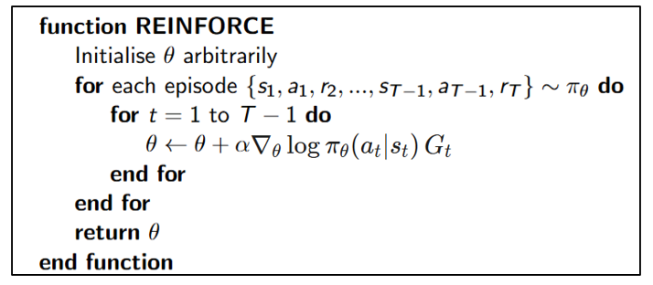
The algorithm above assume that we sample one episode, instead of multiple episodes. Refer to Wikipedia article for multiple episodes sampling.

Okay, let’s get back to the high variance issue. Because we only use a few sampled trajectories instead of the true expectation (which would require infinitely many samples), our gradient estimate becomes noisy. Specifically, we are using Monte Carlo (MC) sampling to sample episodes. To recall equation (1), our goal was to compute \(\mathbb{E}[G_t]\). Basically, we are estimating \(E[G_t]\) relying on MC sampling. Although estimating based on MC sampling offers unbiased estimate, it can produces high-variance estimate ³. The deal is that Monte carlo method waits from the current step to the end of the episode to estimate \(G_t\)

To address this issue, A2C was introduced. They added a Critic network that estimates the value function \(V(s_t)\), which predicts expected return from a state.

\[ V(s_t) \approx \mathbb{E}_{\pi_\theta}[G_t \mid s_t] \]

This value function is updated using Temporal Difference (TD) learning, which involves n-step bootstrapping — updating a guess based on another guess.

\[ G^{(n)}_t = R_{t+1} + \gamma R_{t+2} + \cdots + \gamma^{n-1}R_{t+n} + \gamma R^n V(s_{t+n}) \\ = \sum ^{n-1}_{k=0}\gamma^k R_{t+k+1} + \gamma^nV(s_{t+n}) \]

• real experience: the first \(n\) rewards \((R_{t+1}+ \cdots + R_{t+n})\)
• a guess: the bootstrapped value \(V(s_{t+n})\)

Based on \(G_t^{(n)}\), the update beceoms:

\[ V(s_t) \leftarrow V(s_t) + \alpha(G^{(n)}_t - V(s_t)) \]

You cut off after \(n\) steps and then use the value function \(V(s_{t+n})\), which is your to estimate the ramaining return. What if \(n = \infty\)? Then n-step bootstrapping becomes the MC method. For everything beyond step \(n\), you don’t sample random outcomes but you just plug in the average expected value \(V(s_{t+n})\). Because \(V(s_{t+n})\) is a smooth average over many past samples, it’s much less random than the unrolled future would be. As a result, n-step bootstrapping may introduce small bias but reduce variance.

Going back to A2C, it trains two neural networks simultaneously. The Actor \(\pi_\theta\), which learns the policy, and the Critic \(V(s_t)\), which learns to predict state values and stabilize the policy updates.

\[ V(s_t) = \mathbb{E}_{\pi\theta}[G_t|s_t] \\ A_t = G_t - V(s_t) \\ \]

The difference between the actual return \(G_t\) and the estimated value \(V(s_t)\) represetns how much better or worse the action \(a_t\) performed. This quantity is known as the advantage function \(A_t\). Finally, the gradient of the objective function is

\[ \nabla_\theta J(\theta) = \mathbb{E}_{\pi_\theta} \left[ \nabla_\theta \log \pi_\theta(a_t|s_t) \, A_t \right] \quad (3) \]

I skipped the derivation from euqation (2) to (3). Since the Advantage Actor–Critic (A2C) method was introduced, modern policy gradient approaches typically use this advantage-based formulation instead of the vanilla policy gradient. Now we are ready to move on to PPO.

Proximal Policy Optimization (PPO)

Training language models to follow instructions with human feedback by OpenAI brought Reinforcement Learning from Human Feedback (RLHF) into the mainstream of language model training. We’ve heard about it frequently, but without understanding what Proximal Policy Optimization (PPO) is, we cannot truly grasp how RLHF fine-tunes large language models to align with human preferences.

PPO - Problem of the A2C Policy gradient

PPO is an Actor-Critic algorithm that uses a single neural network with two heads: one for the actor (policy) and another for the critic (Value function) ⁴. In the A2C section, we see that the advantage function \(A_t\) helps reduce the variance of the gradient estimate. However, there is still an issue. Let’s see the quote written in original PPO paper.

While it is appealing to perform multiple steps of optimization on this loss \(\nabla_{\theta} J(\theta)\) using the same trajectory, doing so is not well-justified, and empirically it often leads to destructively large policy updates.

The phrase “using the same trajectory” refers to reusing the exact same batch of experience \(\tau\) collected by the old policy \(\pi_{\theta_{\text{old}}}\).

\[ \text{batch} = \tau = \{s_0, a_0, r_1, s_1, a_1,r_2, \dots\} \]

But something is not right. Once policy gradient is updated, the action and state will be changed, resulting in a new trajectory. Shouldn’t we then collect a new batch (trajectory)? Why people reuse the same batch? Because collecting new trajectories (running the environment again) is expensive. So, practically, researchers often try to reuse the same batch of old data. Okay, now we see reusing the same batch may have some negative impact but still not clear about “it often leads to destructively large policy update”. We are gonna touch base later but first let’s see how they prevent this issue.

PPO - Clipped Surrogate Objective

We know the objective function (eqation (3)) doesn’t work well when performing multiple gradient updates using the same trajectory. The core idea behind PPO is to prevent the policy from moving too far from the old policy while still allowing multiple optimization steps on the same batch.

To fix this, PPO introduces the probability ratio:

\[ r_t(\theta) = \frac{ \pi_{\theta}(a_t \mid s_t) }{ \pi_{\theta_{\text{old}}}(a_t \mid s_t) }. \]

This ratio measures how much the new policy’s probability of an action has changed compared to the old one. If \(r_t(\theta)\) deviates too much from 1, it means the new policy is too different from the old policy.

The clipped version of the PPO objective, Clipped Surrogate Objective, is given by:

\[ L^{\text{CLIP}}(\theta) = \mathbb{E}_t \left[ \min\left( r_t(\theta) A_t,\, \text{clip}\left(r_t(\theta), 1 - \epsilon, 1 + \epsilon\right) A_t \right) \right]. \quad (4) \] \[ \text{clip}(r_t(\theta), 1 - \epsilon, 1 + \epsilon) = \begin{cases} 1 - \epsilon, & \text{if } r_t(\theta) < 1 - \epsilon, \\ r_t(\theta), & \text{if } 1 - \epsilon \le r_t(\theta) \le 1 + \epsilon, \\ 1 + \epsilon, & \text{if } r_t(\theta) > 1 + \epsilon. \end{cases} \]

This prevents the new policy from drifting too far from the old one, effectively bounding the policy update. Intuitively:

• If \(r_t (\theta)\) stays close to 1 → the policy change is small → normal gradient update.
• If \(r_t (\theta)\) moves outside the range → the change is too large → the objective is clipped, stopping further increase in the gradient.

However, Clipped Surrogate Objective is not perfect because clip(r_t(θ), 1−ε, 1+ε) is heuristic, depending on ε. So the authors of PPO introduced another version of PPO.

PPO - KL Penalty (PPO-Penalty)

In another version, PPO penalizes the Kullback–Leibler (KL) divergence between the new and old policy:

\[ L^{\text{KL}}(\theta) = \mathbb{E}_t \left[ r_t(\theta)A_t - \beta\, \text{KL}\!\left[ \pi_{\theta_{\text{old}}}(\cdot \mid s_t) \;\middle\|\; \pi_{\theta}(\cdot \mid s_t) \right] \right] \quad (5). \]

Here, the second term penalizes large deviations between old and new policy distributions. The penalty coefficien \(\beta\) can be adaptively adjusted depending on the distance between old policy distribution and new policy distribution:

\[ \text{distance} = \mathbb{E}_t \!\left[ \mathrm{KL}\!\left( \pi_{\theta_{\text{old}}}(\cdot \mid s_t) \;\middle\|\; \pi_{\theta}(\cdot \mid s_t) \right) \right], \]

\(\pi_{\theta}(\cdot \mid s_t)\) denotes the entire probability distribution over all actions given state \(s_t\), while \(\pi_{\theta}(a_t \mid s_t)\) denotes the probability that the policy chooses a specific action \(a_t\) given state \(s_t\). We update \(\beta\) outside the gradient step using a simple feedback rule:

\[ \beta \leftarrow \begin{cases} \beta / 2, & \text{if } d < \tfrac{1}{2} \times \text{distance}_{target}, \\[4pt] 2\beta, & \text{if } d > 2 \times \text{distance}_{target}, \\[4pt] \beta, & \text{otherwise.} \end{cases} \]

The KL divergence increases when the new policy’s probabilities differ greatly from the old one. Multiplying by \(-\beta\) adds a restoring force that resists large steps away from the old policy.

PPO - Generalized Advantage Estimation (GAE)

In the equation (4) and (5), we saw the advantage function term \(A_t\). However, the authors of PPO didn’t compute the advantage function by \(A_t = G_t - V(s_t)\). Instead, they use Generalized Advantage Estimation (GAE). In A2C section, we learned that \(V(s_t)\) help reduce variance. Depending on a value of \(n\) for n-step bootstrapping, we can set the degree of bias. That being said, it’s still difficult to control the balance between variance and bias because the parameter is discrete and coarse. What if \(n=1\) makes bias too high and \(n=2\) makes bias too low? Can we find some middle point? This is where GAE comes into play, which is give n by:

\[ A^{\text{GAE}(\gamma, \lambda)}_{t} = \sum^{\infty}_{l=0}(\gamma \lambda)^{l}\delta_{t+l} \\ \delta_t = R_t + \gamma V(s_{t+1}) - V(s_t) \]

• When \(\lambda = 1\), it behaves like Monte Carlo (low bias, high variance).
• When \(\lambda = 0\), it behaves like 1-step Temporal Difference (High bias, low variance).

As the parameter \(\lambda\) is continuous, we have more freedom to control the balance. Another benefit of using GAE is that we don’t need full trajectory to estimate \(A_t\). GAE allows computing advantages without waiting for the episode to finish, because it uses bootstrapped estimates from \(V(s_{t+n})\) instead of full return \(G_t\). This is why the authors of PPO chose GAE:

It requires an advantage estimator that does not look beyond timestep. … Generalizing this choice, we can use a truncated version of generalized advantage estimation (GAE). … A proximal policy optimization (PPO) algorithm that uses fixed-length trajectory segments.

Therefore, by training the value function, we can compute the advantage function. The objective function for value network is given by:

\[ L^{\mathrm{VF}}(\theta)= \frac{1}{2} \mathbb{E}_t \left[ \left( V_{\theta}(s_t) -\hat{V}_t^{\text{target}} \right)^2 \right] \]

So, we are training two networks together within PPO, the policy network and value network. The total loss is defined as:

\[ L^{\text{total}} = \mathbb{E}_t \left[ L^{\text{CLIP}}(\theta) - c_1 L^{\text{VF}}(\theta) + c_2S\left[\pi_{\theta}(s_t) \right] \right] \]

where:

• \(c_1\): value loss coefficient
• \(c_2\): entropy coefficient
• \(S\left[\pi_{\theta}(s_t)\right]\): entropy term for exploration

PPO - Reinforcement Learning with Human Feedback (RLHF)

These days, LLM follows three steps training pipeline:

1. Pre-trianing: The model learns general language patterns from large-scale text corpora through self-supervised learning, usually by predicting the next token.
2. Supervised Finetuning (SFT): The pre-trained model is fine-tuned on high-quality instruction-following datasets curated by humans, aligning it more closely with useful and safe responses.
3. Post-training: The model is optimized to refine behavior and better align output using reinforcement learning ⁵.

Reinforcement learning with human feedback (RLHF) is considered to post-training that builds upon PPO. The main idea of RLHF is simple. Instead of traditional supervised finetuing, a human choose a better answer between multiple answers. For example, given two answers:

• Answer A: “The capital of France is Paris.”
• Answer B: “I’m not sure, but maybe France’s capital is London?”

Humans pick A as better. From agent (model) perspective, answer A gives higher reward.

In RLHF frameowrk, four LLMs work in tendom 1) SFT model, 2) reward model, 3) policy model, and 4) value model. The SFT model first provides a well-behaved baseline policy, the reward model evaluates responses based on human preferences, and the PPO model is fine-tuned to maximize those reward scores while staying close to the SFT policy. The value model estimates the expected future reward (value function) of generated responses. They work in tandem so the final PPO-trained policy learns to generate outputs that are both high-quality and human-aligned.

This sounds different from what we just learned about PPO where actor and critic learns the policy. And where does the reward model come from? Didn’t they already obtain ranks of responses based on human preference? Why can we just normalize the rank as score? If we do that, we have two critical problems:

• Normalized rank score shall not be continuous.
• No real environment for exploration.

If the ranks are discrete, we cannot update gradient because it’s non-differentiable. In a standard PPO, reward \(R_t\) is given by the environment. In LLM, there is no external environment giving numeric rewards. Instead, the “environment” is just the prompt (state) \(x\) and the “action” is the text output \(y\). By training reward model on human preference data, \((x, y_{\text{good}}, y_{\text{bad}})\), the reward model will act as an environment. Then should we initialize a new model? We can clone SFT model as it learned prior knowledge in natual language. They removed the token-prediction head and add a scalar regression head that outputs a single real number \(r_{\phi}(x,y)\).

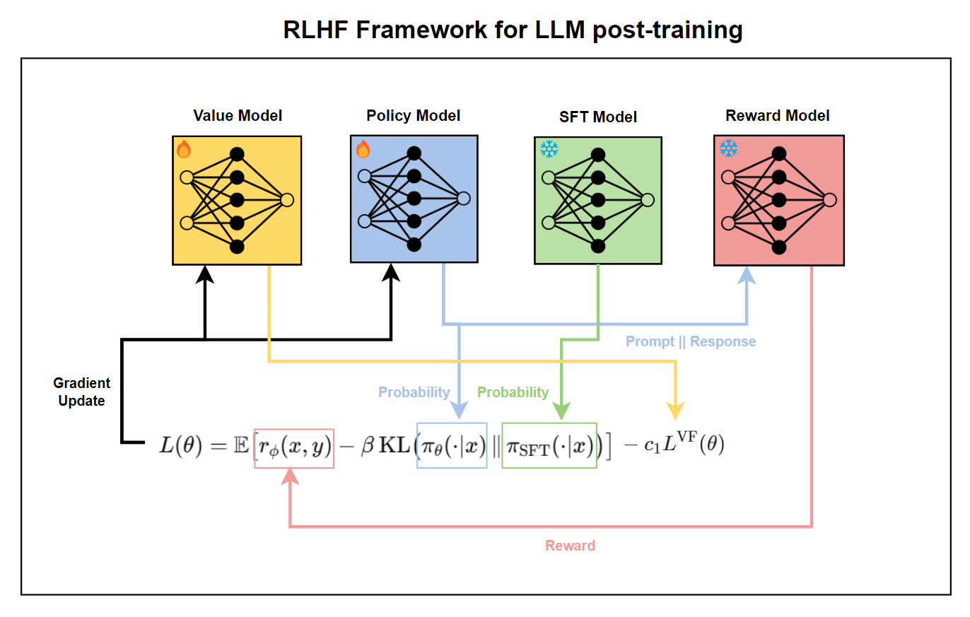
Once the reward model and SFT model are trained, we are ready to train the policy model. The policy model is also an LLM, which is a clone of the SFT model. The value model is initialized from the reward model. During PPO training, the SFT model and the reward model are kept frozen while the policy model and the value model are updated. In the original paper, the total loss function is written as follows:

\[ \text{objective}(\phi) = \mathbb{E}_{(x,y)\sim D_{\pi_{\phi}^{\mathrm{RL}}}}\!\left[r_{\theta}(x,y) - \beta \log\!\left(\frac{\pi_{\phi}^{\mathrm{RL}}(y \mid x)}{\pi^{\mathrm{SFT}}(y \mid x)}\right)\right] \\ + \gamma \mathbb{E}_{x \sim D_{\text{pretrain}}}\!\left[\log\!\big(\pi_{\phi}^{\mathrm{RL}}(x)\big)\right]. \]

The value model \(V_\theta\) and advantage function \(A_t\) are omitted from the total loss function. However, if you see their source code, you can see value function is included.

Generalized Reparameterized Policy Optimization (GRPO)

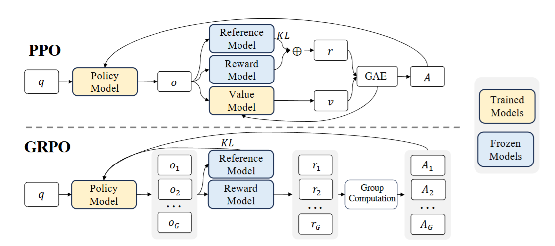
Generalized Reparameterized Policy Optimization (GRPO) ⁶ was proposed to address a heavy computational and memory overhead due to the value function \(V_\theta\). PPO trains two networks simultaneously, the policy network and the value network. However, training two large language models are expensive, demanding a substantial memory. GRPO simplifies the PPO framework by eliminating the value model. Instead, GRPO estimates the baseline from the average reward of multiple sampled outputs for the same question. For a given question \(q\), a group of outputs \(\{o_1, o_2, \dots, o_G \}\) are sampled from the policy model \(\pi^{\text{old}}_\theta\). The reward model scores each output in the group \(\{R_1, R_2, \dots, R_G\}\).

The rewards are normalized by subtracting the group average and dividing by the standard deviation, which becomes an advantage \(A\) at token index \(t\) and sample index \(i\).

\[ \hat{A}_{i,t} = \bar{R}_i = \frac{R_i - \text{mean}(R)}{\text{std}(R)} \]

This makes sense because by the definition, \(A_t\) is the difference between cumulative reward and expected reward. The value of the advantage is constant across all tokens in that output.

\[ \hat{A}_{i,t} = \bar{R_i} \quad \forall t \]

The objective function of GRPO is composed of two terms: CLIP loss and KL divergence loss.

\[ J^{\mathrm{CLIP}}(\theta)= \mathbb{E}_{q,i} \!\left[ \frac{1}{|o_i|} \sum_{t=1}^{|o_i|} \min\!\left( r_{i,t}(\theta) \hat{A}_{i,t}, \, \mathrm{clip}\!\big(r_{i,t}(\theta), 1 - \epsilon, 1 + \epsilon\big) \hat{A}_{i,t} \right) \right]. \]

Here, the probability ratio \(r_{i,t}(\theta)\) ratio denotes how the current policy’s likelihood of generating token \(o_{i,t}\) differ from that of the old policy, conditioned on the prompt \(q\) and the preceding token sequence \(o_{i,\lt t} = (o_{i,1}, o_{i,2}, \dots, o_{i,t-1})\).

\[ r_{i,t}(\theta) = \frac{\pi_{\theta} (o_{i,t}|q,o_{i,\lt t})} {\pi_{\theta _{old}} (o_{i,t}|q,o_{i,\lt t})} \]

Finally, the complete objective function is given by:

\[ J^{\mathrm{GRPO}}(\theta)= J^{\mathrm{CLIP}}(\theta) + \beta \text{KL}\left[ \pi_\theta ||\pi_{\text{ref}} \right] \]

Conclusion

In this post, we traced the evolution of policy-based reinforcement learning from the basic policy gradient to A2C, PPO, and finally GRPO. Each method progressively improved training stability and sample efficiency by addressing variance, bias, and large policy updates. Together, they illustrate how modern reinforcement learning principles have shaped the way large language models are fine-tuned and aligned with human preferences.